Performance in Parallel Programming
Performance Experiments
Let’s measure the performance of our producer/consumer primes counter. I’ve created a version that varies the number of worker threads from 1 to 16. For each worker-thread count, it runs the entire parallel system 10 times and takes the average wall-clock running time. If you want to play along at home, here’s the complete code.
This self-timing program prints things out in CSV format. When I ran this on my machine once, it printed these results:
workers,us
sequential,134134
1,142127
2,73236
3,52692
4,40498
5,36086
6,30115
7,26235
8,24882
9,25613
10,26563
11,27110
12,26788
13,25381
14,26397
15,26917
16,28449
The numbers here are microseconds. I’ve also included, on the first row, the time for a purely sequential version—one with a single thread, no mutexes, no bounded buffers, and no condition variables.
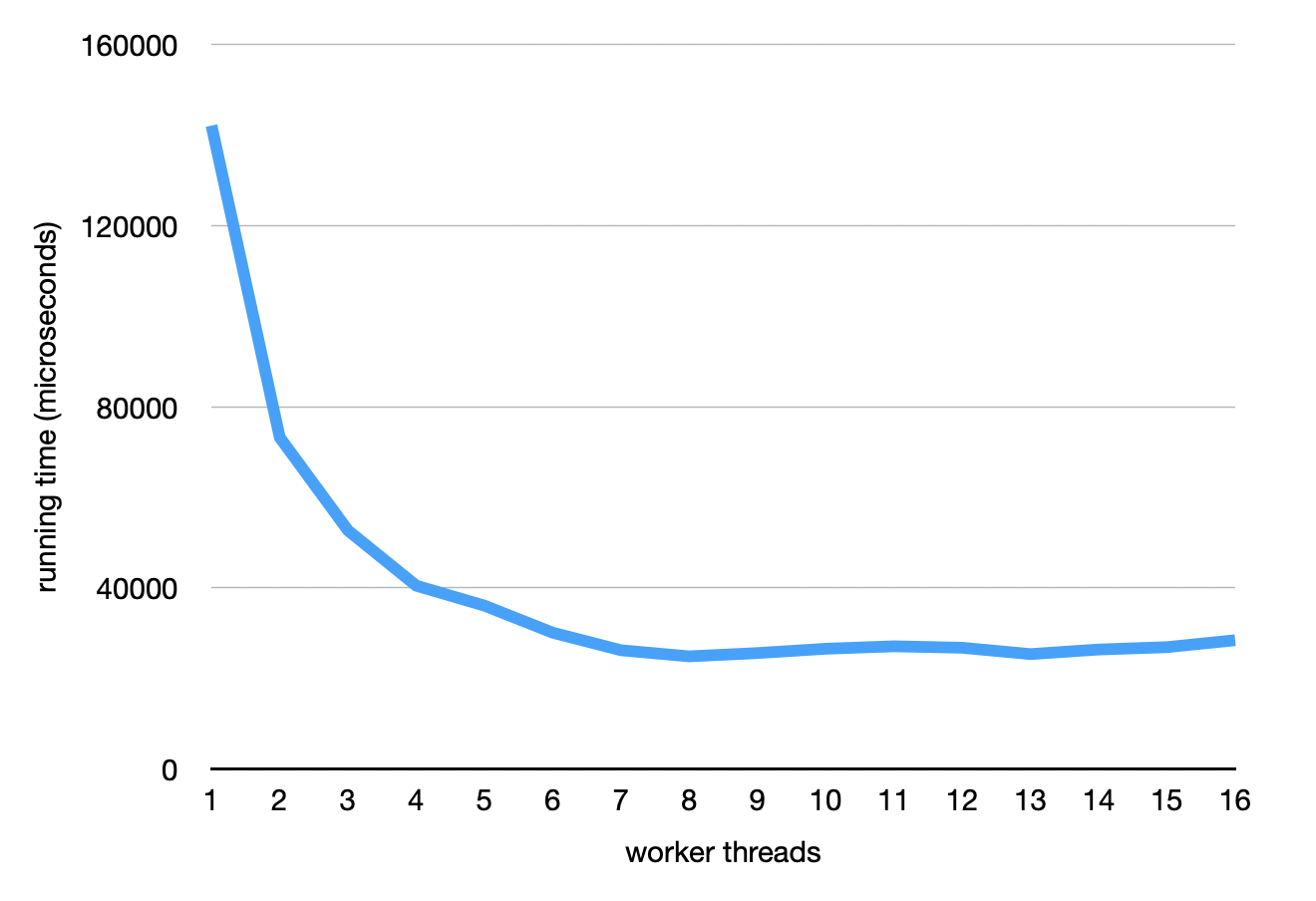
Let’s plot these times:

It looks like adding threads makes the program go faster, which is great. It also levels out at certain point, and maybe even starts to get a little worse. This also makes sense: once we have used up all the parallel hardware resources in my machine, adding more threads doesn’t help, and it can even hurt because the threads need to spend more time synchronizing. The machine I used for this experiment has 8 hardware thread contexts, which is why things don’t get any faster after that.
Speedup and Scalability
Another way to look at this data is to compute the speedup: the ratio you get when you divide the time taken to run on 1 thread by the time taken with n threads. A speedup of 2.0, for example, means that the program ran 2 times faster than the baseline.
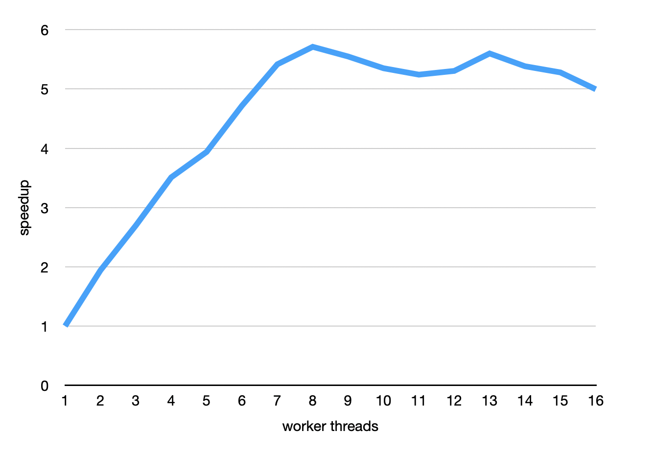
We can plot those numbers too:

Examining the speedup as the number of threads vary tells us about the parallel program’s scalability. If a program gets N× faster when we use N threads, that’s great scalability. When it doesn’t quite hit that ideal, that’s reality—no real software scales perfectly forever.
The chart here shows us that this program scales very well up to 8 threads. The 2-thread exaction is 1.94× faster than the 1-thread version, which is really close to 2. Things slowly deteriorate a little, and the 6-thread version is only 4.72× faster than the 1-thread version. That means this program scales very well but not quite perfectly.
Comparing to a Single Thread
If you measure only scalability, you can miss a really important pitfall in parallel programming: just adding parallelism can come at a cost. It is always therefore important to compare your 1-thread parallel program with a simple sequential baseline.
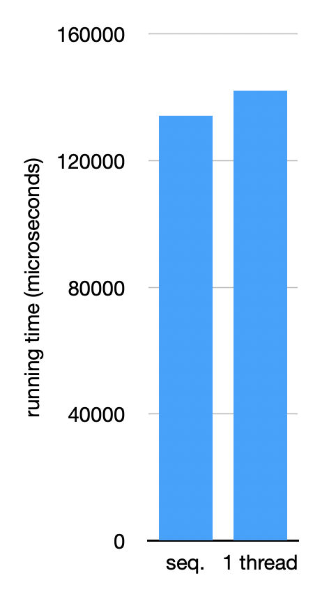
Her’s a simple plot comparing a plain, sequential primality checker with 1-worker version of our producer-consumer implementation:

In this program, the parallel setup costs something, but not a lot. This also makes sense: there is a cost to allocating and coordinating the bounded buffer, and the producer/consumer setup inherently involves some overhead for synchronization. But most of the work is spent on actually running the primality check, so that dominates the running time.
But the cost is not always so small. For an entertaining read about parallel systems that are hilariously slower than sequenial ones, I recommend the 2015 paper “Scalability! But at what COST?”.
Modeling Parallel Performance
The reason this program scales so well is because the problem it’s solving is embarrassingly parallel. An embarrassingly parallel problem is one where you can break it down into completely independent chunks and solve the chunks in isolation, without every communicating between those chunks. Checking whether a single number is prime is a completely independent, isolated piece of work. There is no need for two threads processing different numbers to ever coordinate.
There are many embarrassingly parallel problems in the world, but there are just as many problems that are more difficult to parallelize. It can be useful to generalize the “embarrassingly parallel” concept to characterize how parallelizable a given program is. Imagine two extremes on a spectrum:
- On one side, there are purely sequential programs: ones that need to run on a single thread, and no parallelism can ever offer any speedup.
- On the other side, there are embarrassingly parallel programs: ones where it is trivial to divide up work, and you can roughly expect perfect scalability. In other words, n threads lead to a speedup of roughly n in this ideal case.
All real programs lie somewhere on this spectrum. A common tool for understanding the potential benefit of parallelization is Amdahl’s law. It consists of this formula:
speedup=11−p+ps
where p is the fraction of the program that can be parallelized and s is the amount of parallelism you use. So for a completely sequential program, p=0, and for a perfectly embarrassingly parallel program, p=1.
One important takeaway from Amdahl’s law is that surprisingly tiny non-parallelizable parts of programs can totally ruin their scalability. For example, imagine that 5% of your program needs to run sequentially, so p=0.95. With 2 threads, the results are not so bad: Amdahl’s law predicts a 1.9× speedup. But with 16 threads, the speedup is only 9.1×. Even for a 99% parallel program, if you scale to a 192-core machine, the law predicts a speedup of only 66×.