Chapter 8
Matching Markets
Let us now return to the housing allocation example from the introduction and to the bipartite matching problems we considered in chapter 6. Consider the bipartite graph in Figure 8.1 (which is the same one we considered in the introduction) where we have a set of three people (, , and ) on the left side and a set of three houses (, , and ) on the right side, and interpret the existence of an edge between an individual and a house as saying that the individual finds the house acceptable.
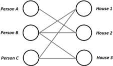
Figure 8.1: A basic example of a matching problem between people and houses.
Using the maximum matching algorithm described in chapter 6, we can find the largest set of players that can be “matched” (i.e., allocated) to a house that they find acceptable (specifically, one such maximum matching would match to , to , and to ). But, in such matchings, we are only guaranteed that the people get some house they find “acceptable.” In reality, however, people have preferences over houses; we may represent these preferences by specifying, for each player, an (individual) valuation for each house. Additionally, houses are typically not free; we may thus also associate prices with each house, and define a player’s utility for a house as their valuation for the house minus the price they would have to pay for it. We refer to such a situation as a matching market. In this chapter, we investigate how correctly set prices—so-called market-clearing prices—can be used to ensure that not only all buyers get allocated a house, but they also end up with their most preferred allocation.
8.1 Definition of a Matching Market
We turn to formalizing the general matching market problem. Given a set of players (buyers) and a set of items (houses) :
- we associate with each player (buyer) , a valuation function .1 For each , determines ’s valuation for item (independent of its price).
- we associate with each item , a price .
- a buyer who receives an item gets utility
(that is, the valuation it has for the item, minus the price it needs to pay); buyers who do not get any item get utility 0.
For simplicity of notation, we restrict to the case when , but the more general case can be reduced to this special case by either adding “dummy buyers” (who value all items at 0) or adding “dummy items” (with value and price 0).
Definition 8.1. We refer to the tuple , where , and is a vector of functions such that for all , as a matching market.
Given a matching market , we are interested in studying different allocations of items to players such that each item gets allocated to at most one player (or remains unallocated). In other words, an allocation is a matching in the complete bipartite graph over players, , and items, . (Recall that in a complete bipartite graph, the edge set is the full set of all possible edges, so that all allocations are possible.)
Definition 8.2. An allocation, or matching, for a matching market is a matching in the complete bipartite graph over .
An outcome of a matching market specifies the allocation as well as prices for all the items ; we specify these prices through a price function , where for every , specifies the price for item :
Definition 8.3. Given a matching market , we refer to the pair as an outcome of if is an allocation for and is a function .
8.2 Acceptability and Preferred Choices
Given a matching market and a price function , we say that item is acceptable to buyer if (i.e., buyer has value for item that is at least its price). We can now define the “acceptability graph” induced by and .
Definition 8.4. Given a matching market and a price function , we define the induced acceptability graph , where if and only if is acceptable to .
The fact that is acceptable to does not imply that prefers over all other items; we say an item is a preferred choice for if is acceptable to and maximizes over all items in —that is,
Note that there may not necessarily exist a unique preferred choice for all buyers; for instance, two items could have the same valuation and price.
The notion of a preferred choice allows us to construct a different bipartite graph:
Definition 8.5. Given a matching market and a price function , we define the induced preferred choice graph as , where if and only if is a preferred choice to .
See Figure 8.2 for an illustration of induced acceptability and preferred choice graphs. We can easily guarantee a perfect matching in the acceptability graph by making all items free ( for all ), since then every item would be acceptable to every buyer (so we can just give the item with index to buyer ). Can we also set prices so that everyone ends up with an outcome they are the most happy with (and not just find acceptable)? That is, can we set prices so that there exists a perfect matching in the preferred choice graph (and thus everyone ends up with their preferred choice)? The notion of a market equilibrium addresses this.
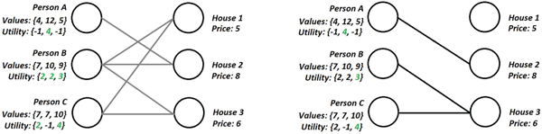
Figure 8.2: Left: The acceptability graph for a matching market and price function . Right: The preferred choice graph for the same , .
Definition 8.6. Given a matching market , we say that an outcome is a market equilibrium (or Walrasian equilibrium) if is a perfect matching in the preferred choice graph induced by and .
The reason we call such a pair, , an equilibrium is that in it, no buyer prefers to switch to a different item (as they are receiving their “preferred choice”) or to not buy their assigned item (as they are receiving non-negative utility for it).
For a given matching market , prices are called market clearing if there exists some market equilibrium of the form for .
8.3 Social Optimality of Market Equilibria
As we now show, market equilibria are socially optimal outcomes. To formalize this, define the social value of an allocation in a matching market as
Note that this notion of social value only takes into account the value the buyers have for the items; in other words, we are implicitly assuming the seller has no value for the items.2 Also, note that the social value is different from the sum of buyers’ utilities, as it considers only the value the buyers get from the items, but without considering the prices they need to pay for them. However, it is not hard to see that the social value of an assignment actually equals the social welfare of all players (i.e., if we consider the utility of both the buyers and the seller) no matter what the prices are, if we define the utility of the seller to be the sum of the prices paid by the buyers. More precisely, define as the sum of the buyers’ utilities + the seller’s utility; namely:
As the prices cancel out in the expression, it simplifies to just
We thus conclude the following claim:
Claim 8.1. For any matching market , any prices and any allocation for , we have that
We say that an allocation maximizes social value if where the is quantified over all allocations for . Similarly, an allocation and and prices maximize social welfare if (where again the is defined over allocations and prices for ). By Claim 8.1, we directly have the following corollary.
Corollary 8.1. For any matching market , an allocation maximizes social value if and only if maximizes social welfare for any (or every) .
Thus, if we have an outcome that maximizes social value, then social welfare will be maximized regardless of how we set prices. Let us now use this observation to show that any market equilibrium maximizes social welfare.
Theorem 8.1 (Social optimality of market equilibria). Given a matching market and a market equilibrium for , we have that maximizes social value.
Proof. Consider some market equilibrium for ; we aim to show that maximizes social value. Toward this, consider some (potentially other) assignment that maximizes social value for . By Corollary 8.1, also must maximize social welfare (in fact, maximizes social welfare for any ). Since is a perfect matching in the preferred-choice graph, by assumption, every buyer must receive an item that maximizes their utility given the prices (and which gives them non-negative utility). In particular, for all (letting and to deal with the fact that may leave some players unassigned), we have:
And thus, the buyers’ combined utilities are at least as high in as in :
Additionally, since in all items are assigned to some buyer, we have that
and thus the seller’s utility is also at least as high in as in . We thus conclude that
It follows that must also maximize social welfare, and then, by Corollary 8.1, we have that maximizes social value as desired.
■
Let us end this section by noting that whereas the proof of Theorem 8.1 is relatively simple, the fact that this result holds is by no means a triviality—we have already seen several examples of situations (e.g., coordination and traffic games) where equilibria lead to outcomes that do not maximize social welfare. Theorem 8.1 is an instance of what is known as the first fundamental theorem of welfare economics and a formalization of Adam Smith’s famous invisible hand phenomenon—that free markets lead to a socially optimal outcome as if guided by “unseen forces.”
8.4 Existence of Market Equilibria
So, given the awesomeness of market equilibria, do they always exist? In fact, it turns out that they always do! Thus, we can always set prices in such a way that (1) everyone gets one of their preferred choices, and (2) items are given to people in a manner that maximizes social value.
We now show that not only do market equilibria always exist, but they can also be efficiently found (relying on the material covered in chapter 6). This theorem is an instance of what is referred to as the second fundamental theorem of welfare economics.
Theorem 8.2. A market equilibrium exists in every matching market . Additionally, there exists an efficient procedure that finds this equilibrium in polynomial time in , where is an upper bound on the valuations of all players.
Proof. We present a particular price updating mechanism—analogous to BRD for games—which will converge to market-clearing prices. Start by setting for all . Next, iteratively update prices as follows:
- If there exists a perfect matching in the preferred-choice graph, we are done and can output . Recall that by Theorem 6.2, this step can be performed efficiently.
- Otherwise, by Theorem 6.3, there exists a constricted set of buyers (i.e., a set such that ) in the preferred-choice graph; furthermore, recall that this constricted set may also be found efficiently.
- Next, raise the prices of all items by 1.
- If the prices of all items are now greater than zero, shift all prices downward by the same amount (i.e., 1, since we can only increase prices by 1 in any step) to ensure that the cheapest item has a price of zero.
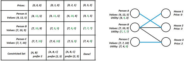
Figure 8.3: The table on the left describes the evolution of the algorithm and all players’ utilities given the current prices; the preferred choices of each buyer are shown in green. The perfect matching in the final preferred-choice graph (i.e., the equilibrium assignment) is shown in blue.
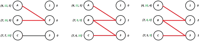
Figure 8.4: The preferred-choice graphs for the intermediate states of the algorithm. Constricted sets are indicated by red edges.
(An example of the execution of this procedure can be found in Figures 8.3 and 8.4.) Clearly, if this procedure terminates, we have found a market equilibrium. Using a potential function argument, we can argue that the procedure does, in fact, always terminate (and thus always arrives at a market equilibrium):
- For each buyer , define as the maximal utility buyer can hope to get for some item; that is, . (Note that if we have a perfect matching in the preferred-choice graph, then this is actually the utility buyer gets in . Also note that the “maximal utility” may be negative if all items are too expensive.)
- Let be the sum of the potentials for all buyers.
- Let be the “maximal utility” the sellers can hope to get. (Again, note that this utility is attained in a perfect matching since all items are sold.)
- Define the final potential as .
Let us first show that the potential is always non-negative.
Claim 8.2. Consider a single iteration of the algorithm where prices get updated from to . Then .
Next, since there always exists some item with price , we know that for every buyer , since may always obtain non-negative “potential utility” by going for this free item. So , and thus .
■
We next show that the potential decreases at every iteration of the algorithm.
Claim 8.3. Consider a single iteration of the algorithm where prices get updated from to . Then .
Proof. Recall that the algorithm first increases the price of the items in the neighbor set, , of the constricted set, , by 1. This increases by . But for each player , it decreases by 1, since they now must pay 1 extra for their preferred item—we here rely on the facts that (a) since there exists some item with price 0, every player has at least one preferred item, thus , and (b) since valuations are integers, if we increase the prices of all preferred choices of by 1, the items will still maximize ’s utility among items (although there may now also exist other items that maximize ’s utility); thus, for all , decreases by 1. For player , remains the same.
We conclude that decreases by , and thus in total changes by . However, by the definition of a constricted set, , and so must decrease by at least 1 during this phase.
Next, if we shift all prices downward by one, will decrease by , but will increase by (by the same logic as above), and so the price shift step has no impact .
■
Finally, notice that, at the start, and
where is any upper bound on the valuations of the players. So, by the above two claims, the procedure will terminate, and it will do so in at most iterations.
■
8.5 Emergence of Market Equilibria
Tatonnement The above proof just shows that market-clearing prices (and hence market equilibria) always exist. But how do they arise in the “real world”? We can think of the process described above as a possible explanation for how they might arise over time. If demand for a set of items is high (there are too many people who prefer those items—that is, we have a constricted set in the preferred-choice graph), then it seems reasonable to assume that the market will adjust itself to increase the prices of those items.
The price shift operation, however, seems somewhat less natural. But it is easy to see that it suffices to shift prices downward whenever all items are too expensive for some buyer (in other words, when the potential utility of some buyer becomes negative) and thus we cannot sell everything off. In such a case, it may seem more natural for the sellers to decrease market prices (e.g., in a housing market, if too many houses remain for sale, the whole housing market starts going down).
In general, these type of market adjustment mechanisms, and variants thereof, are referred to as tatonnement (French for “groping”) mechanisms and have been the topic of extensive research. Whether market-clearing prices and equilibria actually do arise in practice (or whether, for example, conditions change faster than the tatonnement process converges to the equilibrium) is a question that has been debated since the Great Depression in the 1930s.
Buyer-optimal and seller-optimal market equilibria Let us remark that market equilibria are not necessarily unique. Some equilibria are better for the seller, whereas others are better for the buyers. To understand why this can happen, consider the (degenerate) special case of a single buyer and a single item for sale; if the buyer values the item at , then every price can be sustained in an equilibrium (where is the trivial matching where the buyer gets matched with the seller). In particular, setting the price is clearly optimal for the buyer, whereas setting the price is optimal for the seller. A similar reasoning can be applied also in more complicated situations: we can often shift prices by a small—or, as in Figure 8.5, a large—amount while preserving the matching in the market; higher prices will be better for the seller, and lower prices will favor the buyer.
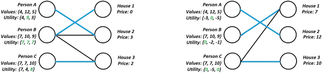
Figure 8.5: Left: The equilibrium we found with the algorithm is, in fact, buyer optimal. Right: If we increase the prices of all houses by as much as possible such that our matching in the preferred-choice graph stays the same (even though the preferred-choice graph now is different!), we obtain the seller-optimal equilibrium. Notice that the seller now gets all of the utility.
8.6 Bundles of Identical Goods
Finally, let us consider a special case of the matching market model, where each “item” is actually a bundle of identical goods. Each player has their own individual value per good , and their valuation for a bundle of size is simply the product of the number of goods, , and their value per good, ; that is,
We assume without loss of generality that the bundles are ordered in decreasing size—that is, . We refer to such a matching market as a matching market for bundles defined by .
Observe that in any outcome that maximizes social value, we have that the largest bundle must go to the person who values the good (and hence the bundle of goods) the most. Consequently, the person who values the good the second-most should get , and so on and so forth. Hence, by Theorem 8.1 (which states that market equilibria maximize social value), this property must also hold in any market equilibrium.
We now show that in any market equilibrium, the largest bundles will also have the highest price per good (i.e., the highest “unit price”). At first sight this may seem counterintuitive—when shopping for groceries we would expect a larger bundle of goods to have a lower price per good! The difference here is that the supply of bundles is limited and each buyer can only purchase a single bundle.3
Theorem 8.3. For any matching market for bundles defined by , and every market equilibrium for , it holds that for every ,
Proof. Consider a market equilibrium . Let be the price per good in bundle . Consider two bundles where , and assume for the sake of contradiction that —that is, the goods in the larger bundle are cheaper. Now consider the player who is matched to the smaller bundle of more expensive goods. His utility is currently , which must be non-negative by the market equilibrium property of . If they were to switch to the larger bundle of cheaper goods, they could increase their utility by , since and by assumption. So cannot be a preferred choice for , contradicting the fact that is a market equilibrium.
■
Notes
Matching markets were first considered by Gale and Shapley [GS62] and the formal model was introduced by Shapley and Shubik [SS71]. Shapley and Shubik [SS71] also proved that existence of market equilibria; the constructive procedure for finding market equilibria is due to Demange, Gale, and Sotomayor [DGS86], and the analysis technique (using potential functions) is due to [EK10]. The notion of a market equilibrium (i.e., a Walrasian equilibrium) and the tatonnement process dates back to the 1870s and the work of Leon Walras [Wal54]. (The treatment of bundles of identical goods is new.)
1We restrict to integer valuations to simplify our treatment; in particular, some of our existence results will rely on this.
2If the seller also has some values for items , this can be captured by introducing an additional “buyer” (representing the seller’s interests in keeping the items) with those valuations.
3The bounded supply assumption is actually only one part of the story here. For instance, another reason why we tend to see lower prices for higher quantity bundles in practice is that values for bundles usually are not strictly linear in the size of the bundle (as we have modeled them here): it is common to have decreasing marginal values.