Lecture 8: Linear Regression

Loading [MathJax]/jax/output/HTML-CSS/fonts/TeX/fontdata.js

Linear Regression

back

In this lecture we will learn about Linear Regression.

Assumptions

Data Assumption:

$y_{i} \in \mathbb{R}$
Model Assumption:

$y_{i} = \mathbf{w}^\top\mathbf{x}_i + \epsilon_i$ where

$\epsilon_i \sim N(0, \sigma^2)$

$\Rightarrow y_i|\mathbf{x}_i \sim N(\mathbf{w}^\top\mathbf{x}_i, \sigma^2) \Rightarrow P(y_i|\mathbf{x}_i,\mathbf{w})=\frac{1}{\sqrt{2\pi\sigma^2}}e^{-\frac{(\mathbf{x}_i^\top\mathbf{w}-y_i)^2}{2\sigma^2}}$

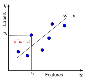
In words, we assume that the data is drawn from a "line" $\mathbf{w}^\top \mathbf{x}$ through the origin (one can always add a bias / offset through an additional dimension, similar to the Perceptron). For each data point with features $\mathbf{x}_i$ , the label $y$ is drawn from a Gaussian with mean $\mathbf{w}^\top \mathbf{x}_i$ and variance $\sigma^2$ . Our task is to estimate the slope $\mathbf{w}$ from the data.

Estimating with MLE

$\begin{aligned} \mathbf{w} &= \operatorname*{argmax}_{\mathbf{\mathbf{w}}} \prod_{i=1}^n P(y_i|\mathbf{x}_i,\mathbf{w})\\ &= \operatorname*{argmax}_{\mathbf{\mathbf{w}}} \sum_{i=1}^n \log(P(y_i|\mathbf{x}_i,\mathbf{w}))\\ &= \operatorname*{argmax}_{\mathbf{\mathbf{w}}} \sum_{i=1}^n \left[ \log\left(\frac{1}{\sqrt{2\pi\sigma^2}}\right) + \log\left(e^{-\frac{(\mathbf{x}_i^\top\mathbf{w}-y_i)^2}{2\sigma^2}}\right)\right]\\ &= \operatorname*{argmax}_{\mathbf{\mathbf{w}}} -\frac{1}{2\sigma^2}\sum_{i=1}^n (\mathbf{x}_i^\top\mathbf{w}-y_i)^2 \\ &= \operatorname*{argmin}_{\mathbf{\mathbf{w}}} \frac{1}{n}\sum_{i=1}^n (\mathbf{x}_i^\top\mathbf{w}-y_i)^2 \\ \end{aligned}$

We are minimizing a loss function, $l(\mathbf{w}) = \frac{1}{n}\sum_{i=1}^n (\mathbf{x}_i^\top\mathbf{w}-y_i)^2$ . This particular loss function is also known as the squared loss or Ordinary Least Squares (OLS). OLS can be optimized with gradient descent, Newton's method, or in closed form.

Closed Form:

$\mathbf{w} = (\mathbf{X X^\top})^{-1}\mathbf{X}\mathbf{y}^\top$ where

$\mathbf{X}=\left[\mathbf{x}_1,\dots,\mathbf{x}_n\right]$ and

$\mathbf{y}=\left[y_1,\dots,y_n\right]$ .

Estimating with MAP

Additional Model Assumption:

$P(\mathbf{w}) = \frac{1}{\sqrt{2\pi\tau^2}}e^{-\frac{\mathbf{w}^\top\mathbf{w}}{2\tau^2}}$

$\begin{align} \mathbf{w} &= \operatorname*{argmax}_{\mathbf{\mathbf{w}}} P(\mathbf{w}|y_1,\mathbf{x}_1,...,y_n,\mathbf{x}_n)\\ &= \operatorname*{argmax}_{\mathbf{\mathbf{w}}} \frac{P(y_1,\mathbf{x}_1,...,y_n,\mathbf{x}_n|\mathbf{w})P(\mathbf{w})}{P(y_1,\mathbf{x}_1,...,y_n,\mathbf{x}_n)}\\ &= \operatorname*{argmax}_{\mathbf{\mathbf{w}}} P(y_1,...,y_n|\mathbf{x}_1,...,\mathbf{x}_n,\mathbf{w})P(\mathbf{x}_1,...,\mathbf{x}_n|\mathbf{w})P(\mathbf{w})\\ & \textrm{As this is a constant it can be dropped. )}\\ &= \operatorname*{argmax}_{\mathbf{\mathbf{w}}} \left[\prod_{i=1}^n P(y_i|\mathbf{x}_i,\mathbf{w})\right]P(\mathbf{w})\\ &= \operatorname*{argmax}_{\mathbf{\mathbf{w}}} \sum_{i=1}^n \log P(y_i|\mathbf{x}_i,\mathbf{w})+ \log P(\mathbf{w})\\ &= \operatorname*{argmin}_{\mathbf{\mathbf{w}}} \frac{1}{2\sigma^2} \sum_{i=1}^n (\mathbf{x}_i^\top\mathbf{w}-y_i)^2 + \frac{1}{2\tau^2}\mathbf{w}^\top\mathbf{w}\\ &= \operatorname*{argmin}_{\mathbf{\mathbf{w}}} \frac{1}{n} \sum_{i=1}^n (\mathbf{x}_i^\top\mathbf{w}-y_i)^2 + \lambda|| \mathbf{w}||_2^2 \tag*{$\lambda=\frac{\sigma^2}{n\tau^2}$}\\ \end{align}$

This formulation is known as Ridge Regression. It has a closed form solution of: $\mathbf{w} = (\mathbf{X X^{\top}}+\lambda \mathbf{I})^{-1}\mathbf{X}\mathbf{y}^\top,$ where $\mathbf{X}=\left[\mathbf{x}_1,\dots,\mathbf{x}_n\right]$ and $\mathbf{y}=\left[y_1,\dots,y_n\right]$ .

A few remarks about the derivation:

$P(y_1,\mathbf{x}_1,...,y_n,\mathbf{x}_n|\mathbf{w})=P(y_1,\mathbf{x}_1,...,y_n,\mathbf{x}_n)$ , because $(y_i,\mathbf{x}_i)$ is independent of $\mathbf{w}$ . Further, $P(y_1,\mathbf{x}_1,...,y_n,\mathbf{x}_n)$ is a constant that does not contain $\mathbf{w}$ and can be dropped from the optimization.
$P(y_1,y_2|\mathbf{x}_1,\mathbf{x}_2,\mathbf{w})=P(y_1|y_2,\mathbf{x}_1,\mathbf{x}_2,\mathbf{w})P(y_2|\mathbf{x}_1,\mathbf{x}_2,\mathbf{w})=P(y_1|\mathbf{x}_1,\mathbf{w})P(y_2|\mathbf{x}_2,\mathbf{w})$ . The first equality holds by the chain rule of probability. The second equality holds because $y_i$ only depends on $\mathbf{x}_i,\mathbf{w}$ and nothing else - so all other terms don't need to be conditioned on. We use this in the more general form $P(y_1,...,y_n|\mathbf{x}_1,...,\mathbf{x}_n,\mathbf{w})=\prod_{i=1}^n P(y_i|\mathbf{x}_i,\mathbf{w}).$

Summary

Ordinary Least Squares:

$\operatorname*{min}_{\mathbf{\mathbf{w}}} \frac{1}{n}\sum_{i=1}^n (\mathbf{x}_i^\top\mathbf{w}-y_i)^2$ .
Squared loss.
No regularization.
Closed form: $\mathbf{w} = (\mathbf{X X^\top})^{-1}\mathbf{X} \mathbf{y}^\top$ .

Ridge Regression:

$\operatorname*{min}_{\mathbf{\mathbf{w}}} \frac{1}{n}\sum_{i=1}^n (\mathbf{x}_i^\top\mathbf{w}-y_i)^2 + \lambda ||\mathbf{w}||_2^2$ .
Squared loss.
$l2\text{-regularization}$ .
Closed form: $\mathbf{w} = (\mathbf{X X^{\top}}+\lambda \mathbf{I})^{-1}\mathbf{X} \mathbf{y}^\top$ .