Machine Learning Projects

Here are write-ups for some interesting machine learning projects I have undertaken. A couple of these have turned into full research projects.

I- Background Modeling and Super Resolution Images Using Bayesian Learning

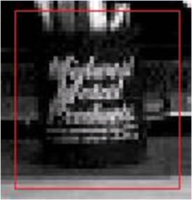
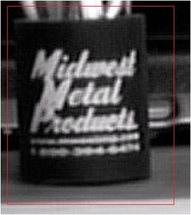
Figure 1: A low resolution shot of a mug.Notice that the writing on the mug is unintelligible.
Figure 2: Applying the reconstruction algorithm on a stream of low resolution images of the mug leads to a higher resolution image. The writing on the mug is now intelligible and reads "Midwest Metal Products".

This project was mostly a reproduction of work done by Peter Cheeseman et al. on high resolution surface reconstruction from multiple images. Their work is desribed in this classical paper.

I- Problem

Given a video stream captured from a camera with a varying pose, we would like to infer a background model responsible for this video. We also aim to extract as much details from the set of images to build a model of the scene at maximal resolution. This is the inverse problem to the one addressed by computer graphics where given complete knowledge of the surface and illumination conditions we can perfectly predict the scene from any perspective. Note that since the camera’s pose is varying, we cannot simply use the maximal pixel frequency technique. However, Bayes’ theorem provides a framework for solving the inverse reconstruction problem.

II- Why Super Resolution is Possible

We are able to get super-resolved models of the surface from the frame sets because each pixel of each frame is a new sample of some location on the actual observed surface. Two frames generated from the exact same camera pose with identical physical conditions produce no net gain from information and hence there is nothing to learn over.With slightly differing camera poses, however, the observed pixel values will be different, and hence we are actually recording information regarding two different patches of this same observed surface. By relating these differences to locations on the surface, it is possible to reconstruct a model grid at a finer resolution than the observation pixilation.

III- A Bayesian Learning Technique Task

Since we know how to solve graphics rendering problem then Bayes’ theorem provides with the formal for solving the inverse problem. To see this we state Bayes’ theorem:

Now let A be the surface model that we are trying to infer along with corresponding physical parameters such as illumination conditions and registration. A is composed of mixels or model pixels. This is to emphasize that mixels are hypothesized. Let B be the graphics or the frames of the video which is our available data. Thus we see that we can find the most likely surface model given our data using maximum a posteriori or MAP since we know the probability of each pixel in each frame given the appropriate physical parameters. We only need to include our belief in the prior.
More precisely we assume that all pixels in all frames are i.i.d. This let us express as a maximum likelihood term:

Now we need to specify the prior. Notice that we can arbitrarily set the scaling factor or resolution of the hypothesized surface or mixels grid. However, such an arbitrariness comes with consequences: The pixels can either underconstrain or overconstrain the mixels grid. In the latter we obtain a plausible surface model. However, in the former the data does not provide enough information to inform us of a surface model at the scaling factor that we have chosen. In this case we need to be cautious of overfitting problems. Thankfully, the Bayesian formal provides us with a solution in the form of the prior. The prior chooses a solution when many equally likely solutions are available. In our case we want to prefer solutions where neighboring mixels are highly correlated. We achieve this by having the prior express the fact that all mixels must be expressed as a linear combination of their neighbors using appropriate weights.
Combining what we have we obtain the posteriori. Maximizing this posteriori with respect to the mixels and physical parameters gives a set of linear equations to solve of the form:

Where omega represent the registration parameters and A represent the neighbor mixels constraint.

IV- Algorithm

Notice that we cannot solve (3) analytically. This is so because to solve (3) we need either exact knowledge of the registration parameters or the mixels, neither of which we know a priori. Therefore, we need to solve (3) numerically be alternating between two steps: First we estimate the registration parameters which we use to estimate the mixels. We keep repeating this bootstrapping procedure until convergence.
It is relatively easy to estimate the registration parameters first. The registration parameters determine the mapping from pixels to mixels and vice versa so that we have for each pixel p:

where is the registration coefficient and is the value of the ith mixel. Since we are assuming that everything that we are seeing is distant then we can assume that we have three degrees of freedom: x, y, and As such to determine the registration matrix , we use normalized correlation between every frame and some random frame that is interpolated to full resolution and that contains all other frames. At this point it is worth mentioning that before such a correlation is computed the random interpolated frame serving as a temporary mixel grid needs to be mandatorily smoothed. This is necessary because this placeholder mixel is quantized which causes pixel sized jump and hence will undermine the scaling of the finer resolution and this will to a hazardous search process. To this end, we use a Gaussian filter which results in a nice smooth mixel grid. Finally to estimate the right angle, to align all images we compute the eigenvector of the placeholder image and that of the frame and take the angle in between.
Once the registration matrix has been computed we can establish our initial mixel grid called the composite using the following formal:

Now use the composite as a starting point to search for the MAP estimate of the mixel grid by solving (3) using the Jacobi method. The update formula used is:

We of course keep updating the terms that need updating until convergence.
As far as data structures, all formulas were implemented using sparse matrices to increase space and time efficiency.

II- Investigation of Reward in Reinforcement Learning

Please see my Research page.

III- Continuous EEG based cursor control using Support Vector Machines and Dynamic Time Warping

Continuous EEG based cursor control has been actively researched in the past two decades for its potential to offer a possibility of communication to individuals with severe paralysis or advanced neurodegenerative diseases. Nevertheless, in our experience, previous research was lacking in two ways: First, all developed control methods were not validated for an extended period of time where a subject is controlling aspects of her EEG signal therefore whether the control model could generalize was not convincingly demonstrated. Second, advanced classifiers such as SVM were not experimented with on large datasets.

In our research we addressed both of these shortcomings. The paper detailing our results can be found here.