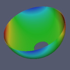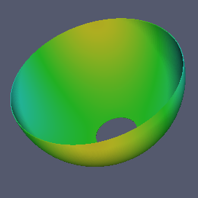
In the second tutorial we work on a hemispherical shell. We will demonstrate how to set fixed boundary conditions.

We will try describe the hemispherical shell shown in Figure hemisphere.png. The origin is located at the center of the shell, and we have four design parameters, \(R\) radius, \(h\) thickness, \(\theta_1\) and \(\theta_2\) which mark the circular shell boundaries, measured from the south pole. The figure is exaggerated for demonstration.
require "mapped_block"

T0 = 300

SILICON = {
   id    = 0, -- unique material id
   E     = 165e9,
   nu    = 0.26,
   rho   = 2330.0,
   kappa = 142,
   alpha = 2.6e-6,
   cv    = 710,
   T0    = T0 } -- T0 on the lhs is a key in material table,
                -- T0 on the rhs is the value from global variable T0


function hemisphere_mesh_generator(R, h, theta1, theta2)
   local function map(x,y)
      local r = R + y*h/2
      local t = pi/2-( (1-x)*theta2 + (1+x)*theta1 )/2
      return r*cos(t), -r*sin(t)
   end
   return mapped_block {
      phi = map,          -- mapping function
      material = SILICON, -- material type
      m = 96,             -- divisions along meridian
      n = 5}              -- divisions through thickness
end
Similar to what we have done with the ring, we define design parameters, create a context, add materials, set stepsize and create mesh gradient.
   R      = 1e-3  -- mean radius
   h      = 1e-5  -- thickness
   theta1 = 15*pi/180  -- angle at the south pole side
   theta2 = 90*pi/180  -- angle at the north pole side


   P = Problem:create{ params  = {R,h,theta1,theta2},
                    m       = 2,
                    name    = "hemisphere", -- optional
                    meshgen = hemisphere_mesh_generator }

   P:add_material(SILICON)

   P:mesh_gradient();

P:write_eps("hemisphere.eps");Now let's say we will have the south circular boundary fixed and the other surfaces free. In the ring example we had a function called free which takes three parameters \(r,z,d\) and returns false to represent free boundary. Setting fixed boundary conditions is implemented by indicating where the fields are going to be zero. Basically we have four scalar fields: radial displacement, angular displacement, axial displacement and temperature change. Zero Dirichlet boundary conditions is indicated as boolean functions. For each scalar field we define an associated list of test functions. If any one of these functions return true at the inspection point, we assume the corresponding component is fixed.
For the ring example wherever the inspection point is, function attached to the boundary condition always returned false, that is to say, nowhere were there a fixed boundary. We should clarify what the input arguments are. \((r,z)\) stand for the inspection point coordinates, and \(d\) is the diameter of the smallest cell in the mesh. We don't need to know its value, yet it is helpful to use it inside the indicator functions as a tolerance value -- direct comparison of floating point values for equality might be dangerous. Since the boundary inspection is done internally by the context, all we have to do is to make sure every indicator function takes \(r,z,d\) as input and returns a boolean value.
Then we pass a table of lists of these function names.
-- A free boundary is not a Dirichlet boundary
function free(r,z,d)
  return false
end

-- We assume the spherical shell is fixed around the boundary
-- on to the pole side. The following coordinates result in coordinates
-- from point 1 to 2 marked on the figure.
function fixed(r,z,d)
  return abs(theta1 - atan2(r,-z)) < 0.01*(d/r)
end

P:set_boundary_conditions{ radial  = { fixed},
                           angular = { fixed},
                           axial   = { fixed},
                           temperature={free} }
Then we can solve for the values we are interested in.
f0 = P:get_eigenfrequency()
BF = P:get_bryans_factor()
Q  = P:get_quality_factor()

print("Frequency      : "..f0)
print("Bryan's factor : "..BF)
print("Quality factor : "..Q)Let's plot the fields on the cross section:
P:write_svg{"disp0.svg"; field=0}
P:write_svg{"disp1.svg"; field=1}
P:write_svg{"disp2.svg"; field=2}
We can output the fields on an underformed 3d mesh in UCD (.inp) file format. You can visualize these files using Paraview.
P:write_inp{"disp0.inp"; field=0}
P:write_inp{"disp1.inp"; field=1}
P:write_inp{"disp2.inp"; field=2}


Could you write a mesh generator which linearly decrease the thickness as a function of \(\theta\) from hmax to hmin?
function thickness_variation_mesh_generator(R, hmax, hmin, theta1, theta2)
   local function map(x,y)
      local t = pi/2-( (1-x)*theta2 + (1+x)*theta1 )/2
      local h = hmin + (hmax-hmin)*(1+x)/2
      local r = R + y*h/2
      return r*cos(t), -r*sin(t)
   end
   return mapped_block {
      phi = map,          -- mapping function
      material = SILICON, -- material type
      m = 96,             -- divisions along meridian
      n = 5}              -- divisions through thickness
end


R      = 1e-3  -- mean radius
hmax   = 2e-5  -- max thickness at theta1
hmin   = 1e-5  -- min thickness at theta2
theta1 = 15*pi/180  -- angle at the south pole side
theta2 = 90*pi/180  -- angle at the north pole side

P = Problem:create{ params  = {R,hmax,hmin,theta1,theta2},
                 m       = 2,
                 meshgen = thickness_variation_mesh_generator }
The rest of the code is similar to the tutorial
Could you change the boundary conditions to include both edges to be clamped?
function free(r,z,d)
  return false
end

function fixed1(r,z,d)
  return abs(theta1 - atan2(r,-z)) < 0.01*(d/r)
end

function fixed2(r,z,d)
  return abs(theta2 - atan2(r,-z)) < 0.01*(d/r)
end

P:set_boundary_conditions{ radial  = { fixed1,fixed2},
                           angular = { fixed1,fixed2},
                           axial   = { fixed1,fixed2},
                           temperature={free} }