
From the point of view of software development, the three most difficult aspects of finite element analysis are the geometric modeling tools, the mesh generator, and the finite element linear system solver. The QMG package is intended to address geometric modeling and mesh generation in three dimensions. It also has a somewhat elementary finite element solver; the sparse matrix solution is handled by Matlab's backslash operator.
The QMG package is embedded in Matlab. The user interacts with it by typing ordinary Matlab commands. All the Matlab functions associated with QMG in matlab begin with the prefix ``gm,'' which is short for ``geometry.'' The functions that begin with ``gm_'' are lower-level ``internal'' functions.
Since Matlab supports only one data type (matrices), geometric objects are represented by arrays whose elements are gibberish to Matlab. These arrays are actually encoded C++ objects.
The geometric modeler and mesh generator can handle polyhedral objects only. A polyhedral object is one that can be constructed by a finite sequence of unions and intersections of halfspaces. (A non-polyhedral object can be approximated by a polyhedral object with many small facets. But there is a very significant penalty in terms of performance of the modeler and mesh generator for many small facets.)
Because the QMG package can handle only flat objects, and because the performance of the mesh generator is not as good as what we'd like, the QMG package is not quite ``professional grade'' software. (In addition, unlike a professional software product, the QMG package comes without warranties and without any promise of support to its users.)
Nonetheless, we believe that QMG package will be useful to researchers in computational geometry and numerical analysis. We believe that there is substantial opportunity in experimenting with and improving many of the underlying algorithms, and indeed, we are interested in future research on improvements.
If you are familiar with mesh generation, here are some of the distinguishing features of the QMG mesh generator that may be different from mesh generators you have used previously. On the positive side,
Structured meshes are a focus of the National Grid Project at the Engineering Research Center at Mississippi State University.
A user of the QMG package typically has two tasks to accomplish:
The geometric model is typically constructed in QMG by calling some of the basic constructors, applying various transformations to the constructed objects, and then applying boolean operations (set union, set difference, etc) to the objects, yielding the final desired shape.
For three-dimensional geometric modeling, graphics are crucial. We rely on the Geomview package from the Geometry Center, University of Minnesota for rendering. If you have your own program that renders polygons in 3D, you can connect it with your own software to QMG.
For the finite element analysis, the user must call the mesh generator, set up the desired boundary conditions, and call the solver program. The boundary conditions are arbitrary matlab functions. They are associated with faces of the domain as property-value pairs of the faces.
Here is an example of solving a two-dimensional boundary value
problem using QMG. This is test file test1 in the
examples directory. The domain is a regular polygon with two holes
and one slit (an internal boundary).
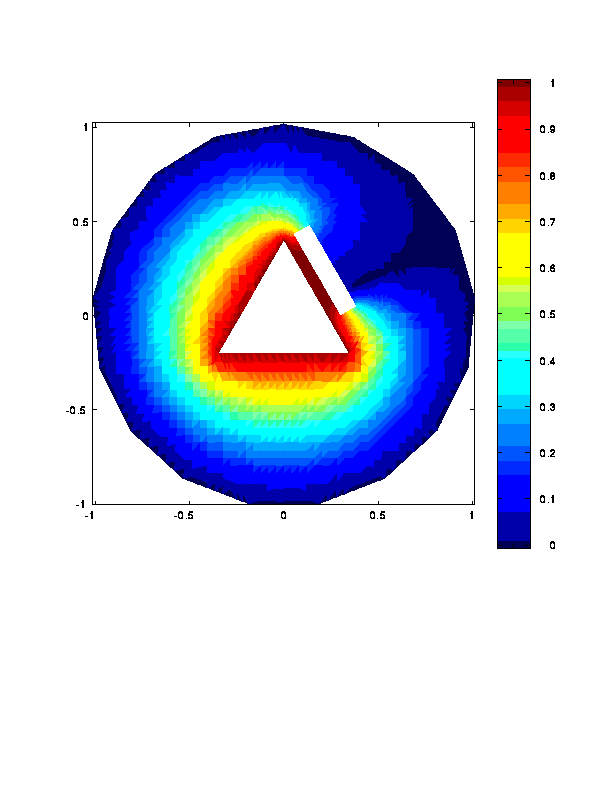
The boundary conditions are u=1 on the exterior face and the slit,
u=0 on the triangular hole, du/dn=0 (insulated) on the rectangular hole.
The user's matlab commands are prefixed with >>.
%% This is an example of a 2D finite element problem with
%% an SL internal boundary.

>> [s,w] = unix('uname -a');
disp(w)
SunOS syn 4.1.3_U1 1 sun4m

>> [s,w] = unix('hostname');
>> disp(w)
syn

>> clock1
1995 may 2   18:24:20

%% Construct an approximately circular region with a triangular hole,
%% a rectangular hole, and a slit.

>> p1 = gmpolygon(17);

>> if exist('interactive')
>>   pause
>> end


%% Rotate the slit so that it is oblique and also subtract
%% it to form an internal boundary.

>> [p,seg,square,c] = gmbasics;
>> eseg = gmembed(seg);
>> t1 = gmrotate(pi/8);
>> t2 = gmtranslate([.4,0]);
>> eseg1 = gmapply(gmcompose(t1,t2), eseg);
>> p2 = gmsubtract(p1, eseg1);
>> if exist('interactive')
>>   pause
>> end


%% Shrink the triangle and make the triangular hole

>> tri = gmpolygon(3);
>> tri1 = gmapply(gmdilate(.2,.2), tri);
>> p3 = gmsubtract(p2, tri1);

>> if exist('interactive')
>>   pause
>> end

%% Make a rectangular hole

>> t1 = gmtranslate(.3,0);
>> t2 = gmrotate(pi/6);
>> t3 = gmdilate(.1,.5);
>> rect1 = gmapply(gmcompose(t1,gmcompose(t2,t3)), square);
>> domain = gmsubtract(p3, rect1);


%% See what we have.


>> if exist('interactive')
>>   domaincolor = gmrndcolor(domain);
>>   gmviz(domaincolor)
>>   gmshowcolor(domaincolor)
>>   pause
>> end


%% Assign boundary conditions.  Put dir. condition of 1
%% on the triangular hole.  Put dir
%% condition of 0 on the outer boundary and the slit.

>> for i = 0:17
>>   domain = gm_addpropval(domain,1,i,'bc', '<d gm_zero>');
>> end

>> for i = 18:20
>>   domain = gm_addpropval(domain,1,i,'bc', '<d gm_one>');
>> end

%%  Put Neumann cond 0 on the rectangular slit.

>> for i = 21:24
>>   domain = gm_addpropval(domain,1,i,'bc', '<n gm_zero>');
>> end

%% Generate a mesh.  Specify 0.2 as the refinement level.

>> clock1
1995 may 2   18:24:26
>> mesh = gmmeshgen(domain,'point2');
>> clock1
1995 may 2   18:24:54

%% Display the properties of the mesh

>> gmget(mesh)
 Type =              simpcomplex
 EmbeddedDim =       2
 IntrinsicDim =      2
 NumSimplices =      856
 NumVertices =       487
 Vertices =          [ (487 by 2) ]
 Simplices =         [ (856 by 3) ]
 SourceSpec =        [ (487 by 2) ]
>> gmchecktri(domain,mesh);

Maximum aspect ratio =      1.427516e+01 achieved in triangle 554, vertices =
 62 ( 0.574109 0.237804)  source = 1/17
 67 ( 0.445326 0.184460)  source = 1/17
 376 ( 0.445326 0.195029)  source = 2/0
Maximum global side length =       2.236968e-01
Minimum global altitude =       2.665202e-03


%% Display the mesh
>> if exist('interactive')
>>   gmviz(mesh,'w')
>>   pause
>> end


%% Solve the boundary value problem.  Conductivity=1 everywhere assumed.

>> clock1
1995 may 2   18:24:56
>> u = gmfem(domain, mesh);
Conductivity on toplev face 0 = gm_one
facet 0 btype = /d/ bfunc = /gm_zero/
facet 1 btype = /d/ bfunc = /gm_zero/
facet 2 btype = /d/ bfunc = /gm_zero/
facet 3 btype = /d/ bfunc = /gm_zero/
facet 4 btype = /d/ bfunc = /gm_zero/
facet 5 btype = /d/ bfunc = /gm_zero/
facet 6 btype = /d/ bfunc = /gm_zero/
facet 7 btype = /d/ bfunc = /gm_zero/
facet 8 btype = /d/ bfunc = /gm_zero/
facet 9 btype = /d/ bfunc = /gm_zero/
facet 10 btype = /d/ bfunc = /gm_zero/
facet 11 btype = /d/ bfunc = /gm_zero/
facet 12 btype = /d/ bfunc = /gm_zero/
facet 13 btype = /d/ bfunc = /gm_zero/
facet 14 btype = /d/ bfunc = /gm_zero/
facet 15 btype = /d/ bfunc = /gm_zero/
facet 16 btype = /d/ bfunc = /gm_zero/
facet 17 btype = /d/ bfunc = /gm_zero/
facet 18 btype = /d/ bfunc = /gm_one/
facet 19 btype = /d/ bfunc = /gm_one/
facet 20 btype = /d/ bfunc = /gm_one/
facet 21 btype = /n/ bfunc = /gm_zero/
facet 22 btype = /n/ bfunc = /gm_zero/
facet 23 btype = /n/ bfunc = /gm_zero/
facet 24 btype = /n/ bfunc = /gm_zero/
>> clock1
1995 may 2   18:24:60

%% Plot the FEM solution

>> if exist('interactive')
>>   figure
>>   colormap(jet)
>>   gmplot(mesh,u)
>>   colorbar
>> end
>> diary off
We now illustrate what this program produced
graphically. The original brep (``brep'' is the
term used for geometric objects in QMG) looks like this.
The edges have been colored so that green corresponds to the insulated
faces, red to the u=1 boundary condition, and blue to the
u=0 boundary condition.
The mesh produced by the mesh generator looks like this:

As seen from the above trace, the worst aspect ratio occurring in this mesh is about 14. It is obvious from looking at this mesh that the mesh generator could ``do better'' in the sense that there are nodes that could be locally displaced to improve the overall quality of the mesh.
We have not implemented any heuristic improvement techniques because our focus has been on three dimensions. In three dimensions we do not know how to heuristically improve meshes.
Finally, the color plot of the finite element solution with mixed boundary conditions looks like this. (Note: in Matlab and postscript the color map has more gradations than the following gif image.)
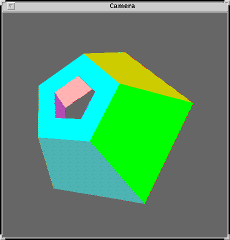
%% In this test, we'll construct a mesh for an interesting
%% 3D shape, that is a tube with an annular pentagonal cross-section.
%% Then we'll triangulate it.  We won't try a boundary value problem
%% this time.

>> [s,w] = unix('uname -a');
>> disp(w)
SunOS syn 4.1.3_U1 1 sun4m

>> [s,w] = unix('hostname');
>> disp(w)
syn

>> clock1
1995 apr 12   16:58:26


>> base = gmpolygon(5);
>> pyr = gmcone(base,[0,0,2]);
>> pyr1 = gmapply(gmtranslate(0,0,-.5),pyr);
>> pyr2 = gmsubtract(pyr,pyr1);
>> pyr3 = gmapply(gmtranslate(0,0,1),pyr);
>> tubeobj = gmsubtract(pyr2,pyr3);
>> gmget(tubeobj)
 Type =              brep
 EmbeddedDim =       3
 IntrinsicDim =      3
 Level0Size =        20
 Level1Size =        30
 Level2Size =        12
 Level3Size =        1
>> tubeobj = gmrndcolor(tubeobj);
>> if exist('interactive') & exist('password')==2 & exist('gm_tclexecute') == 3
>>   eval('gmgeomview(tubeobj);');
>>   pause
>> end

%% Generate a coarse mesh for this object

>> clock1
1995 apr 12   16:58:33
>> mesh = gmmeshgen(tubeobj, 'point4');
clock1
>> 1995 apr 12   17:27:10

>> gmget(mesh)
 Type =              simpcomplex
 EmbeddedDim =       3
 IntrinsicDim =      3
 NumSimplices =      20167
 NumVertices =       4599
 Vertices =          [ (4599 by 3) ]
 Simplices =         [ (20167 by 4) ]
 SourceSpec =        [ (4599 by 2) ]
>> gmchecktri(tubeobj,mesh);

Maximum aspect ratio =      1.122575e+03 achieved in triangle 10482, vertices =
 132 ( 0.622289 -0.511844 0.000000)  source = 1/11
 1464 ( 0.625767 -0.367011 0.082894)  source = 2/7
 3343 ( 0.625767 -0.367011 0.086797)  source = 3/0
 4247 ( 0.625767 -0.444781 0.086797)  source = 3/0
Maximum global side length =       4.268270e-01
Minimum global altitude =       1.504445e-04

>> diary off
The image of the object constructed as shown by Geomview is
This work was supported by the Division of Advanced Scientific Computing of the National Science Foundation through a Presidential Young Investigator grant. Matching funds were received from Xerox, AT&T, Tektronix, IBM, and Sun Microsystems (not all during the same year).
This documentation is written by Stephen A. Vavasis and is copyright (c) 1995 by Cornell University. Permission to reproduce this documentation is granted provided this notice remains attached. There is no warranty of any kind on this software or its documentation. See the accompanying file 'Copyright' for a full statement of the copyright.
example.html,v 1.1.1.1 1995/05/05 01:15:55 vavasis Exp
Stephen A. Vavasis, Computer Science Department, Cornell University, Ithaca, NY 14853, vavasis@cs.cornell.edu