1. Feature Detection

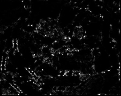
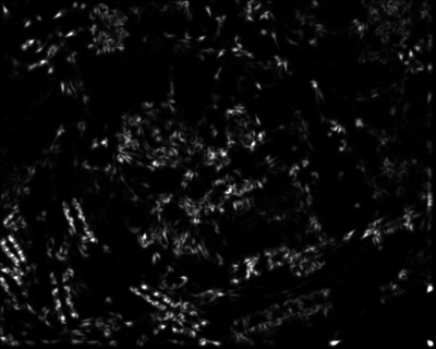
Harris corner detection method is used to identified the gray scale image's points of interest in ComputeHarrisValues. First, the image is filtered by convolving it with a 7x7 Gaussian Kernel to eliminate noises. Then the image derivative in x and y direction is computed by convolving the filtered image with the derivative kernels. Finally compute the Harris matrix H for every pixel, and find the interest point c(H) by dividing the determinant of H by trace of H. Since c(H) is an extremely small number, we multiply c(H) by 100 and set the new value to be the harris value of that pixel. This makes the harris.tga picture more visible and also easier to choose the threshold that is used to compute the local maxima.
The next step is to choose the local maxima by choosing appropriate value for threshold in computeLocalMaxima. Every pixel in the image has a value c computed in ComputeHarrisValues, I choose c to be the local maxima of 5x5 neighborhood. The pixel that has local maxima c greater than the threshold is chosen to be the point of interest. Since Harris corner detection method is invariant to intensity scale but not invariant to intensity shift, the threshold value need to be shift by the same amount that the intensity is shifted. So I find the minimum value among all local maxima and set threshold to be the sum of 0.003 and the minimum value, expecting that if the intensity is shifted, this minimum value is also shifted by approximate the same amount.
The last step is to compute the eigenvector of the largest eigenvalue of the matrix H computed for every pixel. The canonical orientation of the feature is the direction of this eigenvector. Because the image itself already blurred by Gaussian filter, there is no much different between obtaining the feature orientation from eigenvector or from the feature gradient.

2. Feature Description

Three types of feature descriptors completed are: computeSimpleDescriptors, computeMOPSDescriptors, and computeCustomDescriptors.
The computeSimpleDescriptors function simply just takes the 5x5 window centered at the feature location and adds this window to feature data. This is a simplest feature descriptor, it is not invariant to any of the properties. It is expected that this feature descriptor does not perfom well.
The computeMOPSDescriptors is a simplified version of MOPS descriptor. It begins by smoothing the gray scale image with a Gaussian kernel. For each feature, it obtaines 40x40 window centered at the feature location and the direction of feature canonical orientation, then it convolves the window with a Gaussian filter and down-sample to 8x8 window size, and finally adds the 8x8 window to feature data. In order for MOPS to work well and robust, it has to be implemented in multi-scale. However, we do not implement multi-scale here, so MOPS either misses a lot of true postive features or matches almost all true postive features.
The computeCustomDescriptors function is an implemetation of steerable filter. It also begins by smoothing the gray scale image with a Gaussian filter. For each feature, it obtains a 10x10 window center at feature location, then convolve the window with the x and y derivative kernels to obtain the window gradient in the direction of feature canonical orientation. This window gradient is added to the feature data. This is a simple feature descriptor, it is expected to perform slightly better than the simple descriptor.
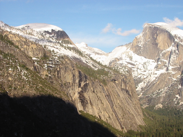
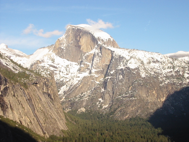
The harris images obtained from the test set graf and yosemite:

Original graf 1 image	graf 1 harris image	Original graf 2 image	graf 2 harris image
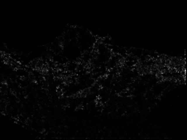Original yosemite 1 image	yosemite 1 harris image	Original yosemite 2 image	yosemite 2 harris image

3. Feature Matching

The only feature matching needs to be implemented is computeCustomDescriptors to assign score for ambiguous matches where the score of a feature in feature set 1 is its SSD distance to its best match in feature set 2 divided by its second best match. The ratio test generally performs better than ssdMatchFeatures, however, ratio test matches the feature wells in higher threshold where SSD distance can give some matches at lower threshold although they might not be correct. The ratio test is more robust than SSD distance.

4. Extra Credit

Inspired by the power of ratio test, I implemented twoRatioMatchFeatures where the idea is the same as ratio but in this feature matching, it also computes ratio of second best distance divided by the third best distance. The score of the feature match is 0.8*(best/second best) + 0.2*(second best / third best). As expected, it performs even better than ratio test with SIFT descriptor for both graf and yosemite test pairs.

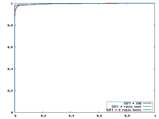graf SIFT feature matching	yosemite SIFT feature matching

5. Performance report

It is obvious that SIFT perfoms better than all 3 descriptors. There are some significant different between ssd distance and ratio test where the ratio test performs much better. MOPS either has very little (close to 0) true positive rate) or very high positive rates this is again is the problem of not doing multi-scaling. Non-scaling MOPS probably requires larger threshold to match features correctly. In addition, MOPS probably needs Non-maximal adaptive suppression method to eliminate the features that very similar to their neighbors.

graf ROC curves	yosemite ROC curves

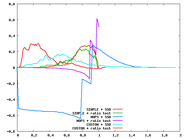
Here are the threshold curves of the descriptors and matching types.

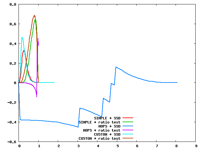graf threshold curves	yosemite threshold curves

In general, performance of MOPS descriptor on the benchmark test sets is not as good as it supposed to be due to the lack of scaling. Custom descriptor - steerable descriptor performs better in most the cases. The different between ssd and ratio test is very significant which implies that there are many ambiguous matches in the data set and the ratio test helps clear this out. We can't really see the significant difference between ratio test and the 2 ratio tests (extra credit) probably due to the problem of the descriptors themselves cannot capture the invariance of features in images as good as SIFT.

bikes data set	Simple descriptor	MOPS descriptor	Custom descriptor
ssd match features	0.350847	0.237046	0.385985
ratio match features	0.510522	0.252641	0.562909
2 ratio match features	0.506897	0.251912	0.559808
graf data set	Simple descriptor	MOPS descriptor	Custom descriptor
ssd match features	0.63027	0.403567	0.49836
ratio match features	0.507244	0.332007	0.527187
2 ratio match features	0.510464	0.368479	0.527619
leuven data set	Simple descriptor	MOPS descriptor	Custom descriptor
ssd match features	0.090903	0.085702	0.110292
ratio match features	0.507252	0.235719	0.482009
2 ratio match features	0.497275	0.231686	0.477939
wall data set	Simple descriptor	MOPS descriptor	Custom descriptor
ssd match features	0.157162	0.165642	0.252964
ratio match features	0.536996	0.201587	0.52251
2 ratio match features	0.535597	0.215594	0.523139

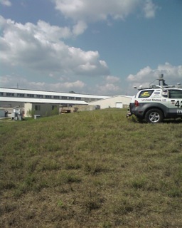
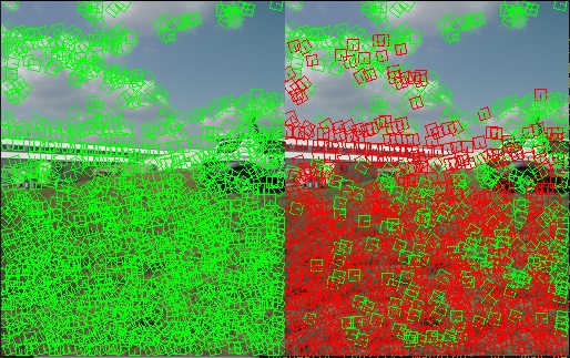
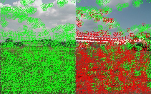
6. Some other testing images

Original Image	Matching with ifself under MOP descriptor	Matching with ifself under custom (steerable filter) descriptor
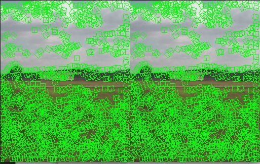Original Image	Matching with ifself under MOP descriptor	Matching with ifself under custom (steerable filter) descriptor