Computer Vision, Spring 2011

Project 1:  Feature Detection and Matching

Wenlei Xie (wx49)

1. Custom Feature Descriptor and Explanation

A simplified and modified SIFT Feature Descriptor is used in this project as the custom descriptor. It mainly followed the SIFT descriptor on the slides.

We choose the SIFT Feature mainly because it has been demonstrated as one of the most successfully feature descriptors in Computer Vision. Its main idea (the combination of histograms) is simple but powerful, which is intuitively robust to several kinds of change, e.g. change of illumination.

Here is the detailed procedure for this custom descriptor.

1) Take a 16x16 square window around the detected feature. The square window’s edge is parallel to the dominant orientation of the feature point.

2) Rotate the window to the horizontal. This operation is to make this feature rotation invariant.

3) Apply the Gaussian filter for the pixels in the window. This implementation used a 3x3 Gaussian mask with. This operation is to make this feature more robust to noise, as the Gaussian filter will soften the patch and thus reduce the effect of the noise points.

4) Calculate the gratitude for each pixel; throw out these pixels with gradient magnitude below a certain threshold. (The threshold is 0.001 in this implementation). This operation is to ignore these pixels that don’t have discriminative information.

5) Divide the 16x16 window into 4x4 grid of cells, i.e. each grid is a 4x4 small window.

6) Compute the orientation histogram for each grid. The orientation is discretized into 8 categories, i.e. the angles in are considered as the same.
In the implementation, we use a ‘soft histogram’, this is to say, for an angle in category i, we add dimension i by 2 while also adding dimension i-1 and i+1 by 1. This is to ‘soften’ the dimension, as the adjacent dimensions are still related.

7) Combine these histograms together. For each grid, there are 8 orientations, thus the descriptor has 16x8=128 dimensions.

2. Performance Report

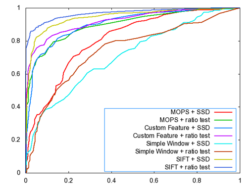
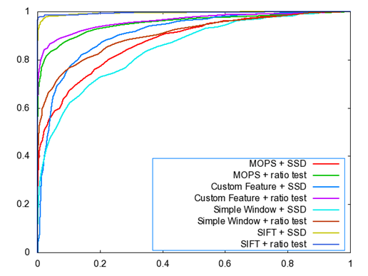
2.1 ROC Curves and AUC result

· Graf Dataset

	AUC
Simple Window + SSD	0.710248
Simple Window + Ratio Test	0.740930
MOPS + SSD	0.808540
MOPS + Ratio Test	0.898305
Customer + SSD	0.903622
Customer + Ratio Test	0.919961

· Yosemite Dataset

	AUC
Simple Window + SSD	0.846409
Simple Window + Ratio Test	0.903634
MOPS + SSD	0.877682
MOPS + Ratio Test	0.951950
Customer + SSD	0.909553
Customer + Ratio Test	0.960553

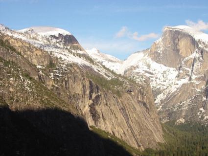
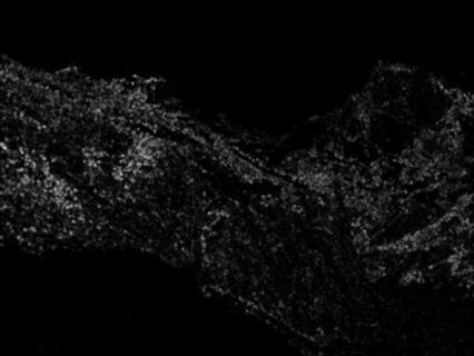
2.2 Harris Score

The Harris Score on Graf

The Harris Score on Yosemite

2.3 Average AUC on Benchmark sets

	Graf	Leuven	Bikes	Wall
Simple+ SSD	0.542540	0.251648	0.284568	0.270532
Simple + Ratio Test	0.539316	0.519957	0.474922	0.538836
MOPS + SSD	0.562743	0.593044	0.630684	0.582338
MOPS + Ratio Test	0.587625	0.656019	0.622528	0.623670
Custom + SSD	0.587297	0.510180	0.579308	0.599822
Custom + Ratio Test	0.605696	0.650979	0.619982	0.629150

3. Strengths and Weakness

As we can see in the ROC curve part, our custom descriptor outperforms the simple MOPS feature implemented in this project, which demonstrates that the combination of gratitude orientation histogram could be used as a very good feature descriptor. Since it only counts for the frequency of gratitude orientation, it is robust to transformation of the pictures.

However, in the benchmark part, we found the MOPS descriptor performs as well as, or even better than the custom descriptor. The main reason is that this implementation of SIFT only use the 16x16 window near the feature point, thus it might not lose some useful information, especially when the picture is foggy, or the pictures have largely different scale, rotation, etc. One might expect a better performance after adding the Gaussian pyramid into this descriptor, which will make this descriptor scale-invariant.

4. More Pictures and Results

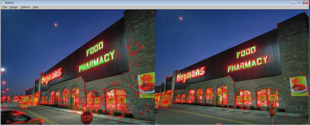
The features on text FOOD PHARMACY are selected to perform the query. The result is good: many features on the corresponding text in the other picture are fetched; while relatively a few mismatched features are found in the other place of picture.

This time we select the text Wegmans instead, and use the alternative picture to provide features. The result is still reasonable but not as good as the previous one. More mismatched features are found. The might be caused by (1) the text Wegmans on the second picture has a large rotation angle and make the descriptors different; (2) some of the features might overlap in one picture but not overlapped in the other. A scale-invariant feature might perform better in this situation.

This query performance is bad. In fact all the selected features in the first photo have its corresponding features in the second photo. However most of them are wrongly matched to other random features. One reason is that some features on the building are similar. Moreover, the direction of the maximum eigenvalue sometimes fails to indicate the right direction in rotation transformation case.

This pair of pictures is taken on different time for the McGraw Tower to test the effect of different illumination. As the result shows, this descriptor can handle the photos with different illumination to some extent. As some of the features on the clock surface are successfully discovered.