CS 6670 Computer Vision, Spring 2011

Project 1: Feature Detection and Matching

---

Tsung-Lin (Chuck) Yang ty244@cornell.edu

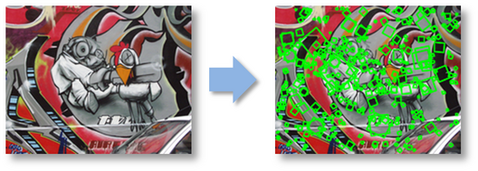
Quick Links: Custom Descriptor Design Choices Performance Strengths and Weakness Others

---

Custom Descriptor

The goal for the feature descriptor is to have a way to represent a feature in order to be used in the matching process later on in the stage. A 45x45 window centered around the feature detected is rotated and downsampled to 9x9 patch. The custom descriptor that I made is of the SIFT descriptor and MOPS descriptor. The steps of generating my custom descriptor is following:

• Prepare for downsampling.

This involves gaussian smoothing the grayscale input image with a 7x7 gaussian kernel. A transformation matrix is needed for transforming sampling location from horizontal to the feature's patch orientation. The transformation matrix is:

T =	cos(angle) -sin(angle) x sin(angle) cos(angle) y 0 0 1

• Determine the downsampled pixel location at the orignal 45x45 window.

Next is to loop through the 9x9 patch window to sample the original image. The applyHomography was called to perform transformation between the feature patch and original image. It also rotates the patch to the dominant gradient angle. Following psudocodes gives you an idea of the process:

loop through 9x9 window (MOPS_WINDOW_SIZE = 9, j++, i++)
mx = (i-(MOPS_WINDOW_SIZE-1)/2)*5;
my = (j-(MOPS_WINDOW_SIZE-1)/2)*5;
applyHomography(mx, my, u, v, T);
save value(u,v) of original image to value(i,j) of temperary patch

• Find the gradient vectors.

Divide 9x9 window into 9 division, so it became 3 big blocks each side. Then find the gradient vectors by finding eigenvalues and eigenvectors just like in the computeHarrisValues. Then build a histogram in each division by using eigen value and eigen vector to project onto 8 directs using following equation:

eigenvalue*cos(theta-eigenvector)


• Store the patch into FeatureSet.

Store the histogram with magnitude in 8 directions into the data field of Features.

Design Choices

My implementation is closely related to the lecture slides. However, there are some difference:

• Patch downsampling selection instead of original patch rotation.

Each feature patch was generated by determining where the resulting pixel coordinate located in the original image. This prevents gaps or out of window pixel from apearing.

• 9x9 window size for feature patches instead of 8x8.

9x9 window size was used for center pixel selection.

Performance

The performance of my implementation can be evaluated by using benchmark as command line argument and benchmark with provided image sets. Each image set aims to identify the most difficult problem in feature detection and matching. The provided image sets includes:

Yosemite	Translation
graf	Perspective/Skew
leuven	Illumination
bikes	Blurring
wall	Perspective/Scale

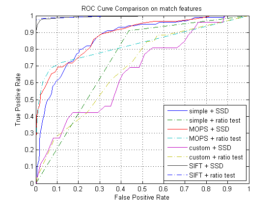
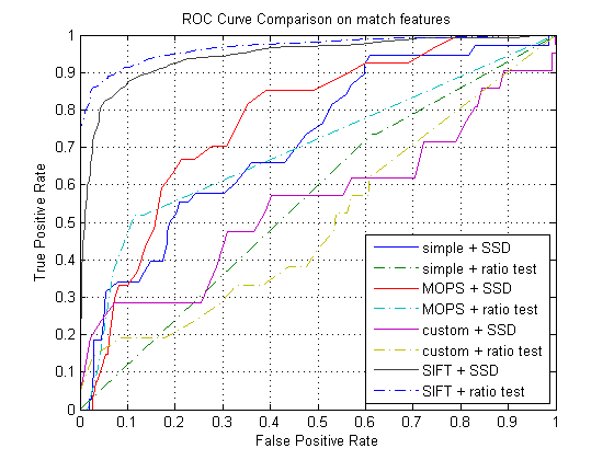
ROC curves on given image sets

• Yosemite



• graf

Harris Operator Results

• Yosemite

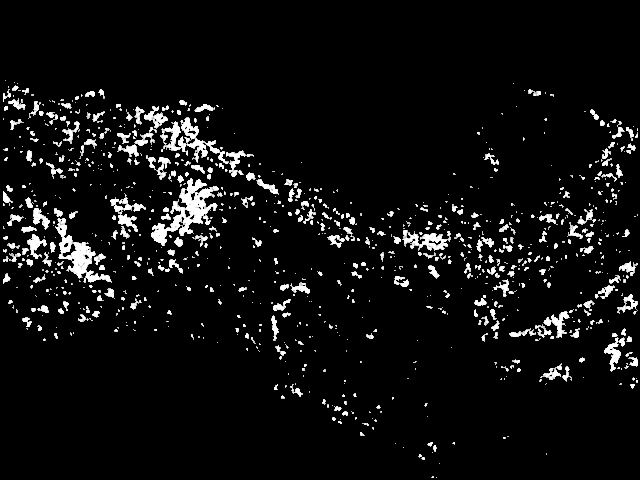
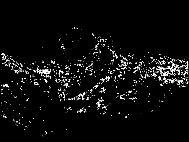
img1 harrisImage	img2 harrisImage

• graf

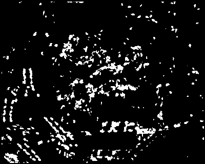
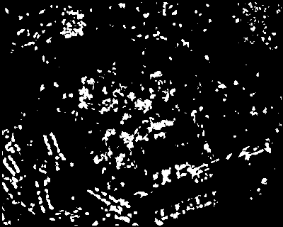
img1 harrisImage	img2 harrisImage

Benchmark Results

Image set	Challenge	Avg. Error(pixels)	Avg. AUC SSD	Avg. AUC Ratio
graf	Perspective/Skew	38.404517	0.296314	0.289008
leuven	Illumination	333.829547	0.110459	0.424730
bikes	Blurring	291.833798	0.479446	0.522791
wall	Perspective/Scale	364.706387	0.314215	0.511421

Strengths and Weakness

As Shown in the ROC plots above, the custom descriptor has higher false postive rate and smaller AUC comparing to SIFT features. Which is kind of expected, I didn't think I implemented it the SIFT like descriptor correctly. Among the two feature matching method, the ratio test yields better true positive rate and more AUC score usually. In the benchmark image sets, the average AUC scores showed how the custom descriptor performs. In graf image set, the average AUC is only 0.296 which shows that my custom descriptor implementation is weak in handling perspective/skew difference. When benchmarked on the bikes, the average AUC score was the highest; this shows that my custom descriptor implementation performs better when handling blurring differences.

Others

I tried the MOPS feature detection and matching that I implemented on the picture that I took. But note that I do not know the homography matrix of the two images, so I couldn't plot the ROC curve to compare the performance. So I plotted the features detected and the matches in between the features visually on the picture and here is some result:

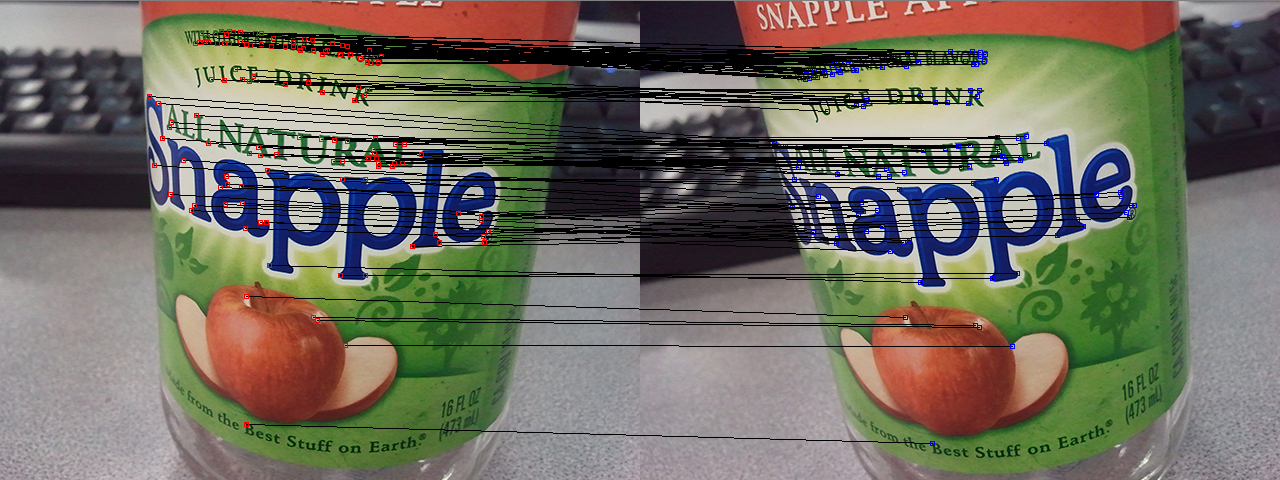
In this image, I slightly rotated the camera with an angle, and it turns out that the MOPS works great when there are lots of distinct features to track and it is easier for it to match correctly.

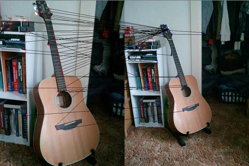
In the image above, I tried to capture the guitar at a different distance resulting a difference in scale. But the result was bad because of the ambiguous features detected around the guitar fret.

In the image above, I blurred the second image. But the performance wasn't very good as I took away many features in the image.