For this project, I implemented one feature detector, two feature descriptors, and one feature matching routine.
My custom feature descriptor is similar to MOPS, but uses two different downsampled patches taken from around the feature point in order to obtain attributes to describe the feature. First, it uses the orientation found by the feature detector to select a 51x51 pixel region around the feature. After rotating this patch such that the orientation is horizontal (theta = 0), we blur the patch using the 5x5 Gaussian filter and subsample down to a 10x10 patch. Each of the pixel values are then normalized and used at attributes to describe the feature. Next, we repeat the process, subsampling down to a 4x4 patch, which is then normalized and features are extracted.
I chose to implement my custom descriptor in this way in order to better detect image scaling. The simplified MOPS descriptor we implemented assumes that images are not scaled, choosing a single size region around the feature and subsampling it. By subsampling twice, additional descriptive features are extracted that help to isolate the features.
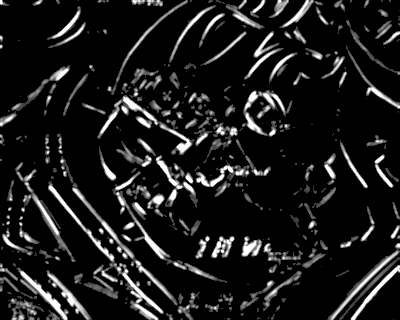
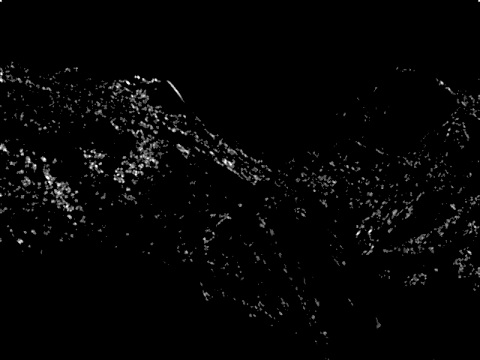
Below are Harris images output when computing features on the graf image img1.ppm and the yosemite image yosemite1.jpg, respectively.


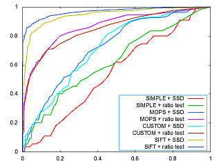
Below are the ROC curves for the Graf and Yosemite data sets, followed by the AUC values for that data


| Graf | Yosemite | |
| Simple Descriptor, SSD Matching | 0.544594 | 0.900788 |
| MOPS Descriptor, SSD Matching | 0.719160 | 0.913043 |
| Custom Descriptor, SSD Matching | 0.716981 | 0.887746 |
| Simple Descriptor, Ratio Matching | 0.620077 | 0.884697 |
| MOPS Descriptor, Ratio Matching | 0.863987 | 0.961527 |
| Custom Descriptor, Ratio Matching | 0.846150 | 0.947203 |
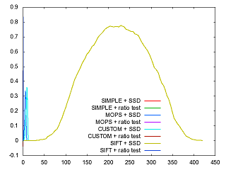
Below are the Threshold curves for the Graf and Yosemite data sets, respectively.


The algorithms were tested on the benchmark dataset, and produced the following average AUC values
| Graf | Bikes | Leuven | Wall | |
| Simple Descriptor, SSD Matching | 0.385637 | 0.403954 | 0.275624 | 0.368451 |
| MOPS Descriptor, SSD Matching | 0.536915 | 0.482561 | 0.660924 | 0.520319 |
| Custom Descriptor, SSD Matching | 0.561591 | 0.630209 | 0.652368 | 0.598114 |
| Simple Descriptor, Ratio Matching | 0.536915 | 0.482561 | 0.532852 | 0.520319 |
| MOPS Descriptor, Ratio Matching | 0.569605 | 0.665497 | 0.693331 | 0.676211 |
| Custom Descriptor, Ratio Matching | 0.565439 | 0.654816 | 0.696620 | 0.644102 |
In addition to the provided datasets, I snapped a couple pictures of a pen on different background to see how the feature matching would be able to find the pen. Below is a sample comparison of results. Without the homography files, ROC plots couldn't be made, but visually their appears to be features matching in a beneficial way. Playing with the threshold value in the non-maxima suppression routine may allow more matches with the addition of more false positives.

The biggest strength that this approach is the ability to pick a large number of interesting features in the images along with orientation. However, the descriptors are not strong enough to reliably make matches between two images. A large number of false positives are reported when testing images in the GUI and object don't seem to be recognized very well. The MOPS descriptor implementation in this assignment is rotation and translation invariant, but is not scale invariant. The custom descriptor attempts to solve that issue somewhat, but is nto a perfect remedy. The algorithms excel most when there is little change in scale and focus entirely on rotation and translation.