
figure 1: Data exchange cases.
| Group number and name: | [5] MIA |
| Team members: | Benjamin D. Cichy, Paul W. Coleman. |
| Task number and name: | [1] Data Exchange |
The goal of our project was to move data through a network over IP. When talking on the telephone to a friend, the voice data (i.e. the sounds that you speak) are transported over the telephone network to the listener at the other end of the phone line. Similarly, data exchange transports voice data between computers involved in a conversation, or between a computer and the gateway.
figure 1: Data exchange cases.
In the MIA system voice connections can be any combination of the 3 cases seen if figure 1. Case A, the simple case, is already implemented in the regular phone system. Case B is when a person on a phone is talking to someone on a computer. Case C is what is generally know as internet telephony -- someone on a computer talking with someone on another computer.
The existing phone system guarantees a certain quality of service (QoS). This is obvious because we hardly ever experience poor quality or get disconnected when on the phone. In order for MIA to be viable we must achieve the best QoS possible, but this is no easy feat. Guaranteeing QoS on the internet is practically impossible. This is most noticeable when downloading a web page; sometimes the page never loads, other times the page downloads in a bursty fashion. Imagine a phone conversation where some words were omitted, or where sometimes people spoke really fast, and then other times they slowed down. This is undesirable, and results in a low QoS. It is our job to hide the undesirable effects of the internet and make QoS as high as possible while transferring voice data over the internet.
The factors that comprise QoS are data loss, latency, and jitteriness. Data loss occurs when the receiver needs to playout some data but there is no data appropriate to play at that time. Latency is the amount of time between the speaker speaking and when the receiver hears what was spoken. The aim is to reduce latency as much as possible; usually for a phone conversation latency under 200ms is acceptable. Finally, jitteriness is the burstiness of the playout. Data exchange regulates the playout so the burstiness of the internet is hidden and playout occurs at a constant rate. How do we optimize all of the factors comprising QoS?
To reduce data loss we used a technique called Forward Error Correction (FEC). FEC sends redundant information in each packet. When a packet is lost we can then reconstruct the data that it contained using information from previous correctly received packets. At the sender each packet we send contains data for a certain time instance. For FEC we add redundant data to this packet from preceding packets. At the receiving side, if the a packet is detected as lost we use the redundant data to reconstruct the lost packet. Because packets are not lost often the redundant data that we send need not be the best quality. Also, packet loss is bursty; when one packet is lost it is likely that more packets will be lost. The average number of sequentially lost packets is two. For this reasons we send redundant data for the preceding packet, and the one before that one. This is best seen in the table below.
|
Group
|
|
|
|
|
Bytes
|
|
|
|
| Time | X | X | X |
It is important to realize that each of the groups represents the same length of time (X), but at different instances. For example, G1 could be the data for time 60 to 80ms. Given this, G2 would then represent a medium quality version of the data from 40 to 60ms. And finally, G3 would be a low quality version of 20 to 40ms. Note that the medium quality version requires half the size of the high quality version, and the low quality version requires only one quarter of the high quality versions size. Basically to make the medium quality data we use every even byte from its high quality versions. The low quality data is every even byte from the medium quality version. This implies that if the high quality data is sampled at 8KHz (as the MIA system is) the medium quality data is sampled at 4KHz, and low quality is 2KHz.
Reducing Latency without Jitter
In order to reduce latency it is important to understand what makes latency high. On the sender side there is some overhead required to create the FEC. Additionally, time is spent sending the data across the network. Also, like the sender, the receiver takes time to handle the packet. These all compound to produce the end to end latency. We have no control over the the actually network performance, so we can't hope to reduce its latency, rather we just accept what it gives us. To reduce the processing overhead the code is carefully written.
What happens if the latency varies over time, which is does? If playout the data when we receive it sometimes data will be played out faster than others based on the varying latency. To resolve this you can stipulate a latency (L). This means that when data is requested data exchange blocks until the current time is greater than packets sending time plus L. This is nice because if the actual latency varies playout won't be affected because the latency is set to L, and playout will be jitter free.
This solution introduces an obvious problem, what value do we use for L? We want to reduce the latency, but it can't be lower than the actual latency in the system. The solution that data exchange uses is called adaptive playout. Adaptive playout dynamically selects the value for L based on the measured latency and the previous value for L. The formula is given below:
This is a low pass filter (smoothing function) allowing the new value of latency to be a based on the weighted old latency and the measured latency. Alpha can be varied for different effects; low alpha puts a higher dependence on the measured latency, but might result in rapid fluctuations; high alpha means that the latency changes very slowly over time. This may result in inappropriate values of L if the latency conditions change and L can't keep up with the changes. Beta is an inflation factor.
The key is to select values for alpha and beta such that minimum latency is optimized. Note this is a trade off between lower latency and waiting to receive all data before playing it out. Figure 2 below shows a theoretical histogram of packet arrivals. No packets arrive before the minimum latency. Most packet arrivals are clustered around a certain time, others take a "long" time to arrive. Alpha and beta should be selected such that at least 90% of the packets arrive before the latency expires.
figure 2: Optimal latency assignment
Time synchronization of machines involved in voice communication is important because the voice data must be replayed at the correct time. A simple example of this is, if party A asks a question and party B replies, the question must precede the answer. The main question to answer is, what granularity of synchronization is needed, and how much overhead can we allow for the synchronization? A high overhead, fine grained solution is RTP. A lighter solution is an initial synchronization at the time of connection start up. The latter solution occurs no overhead during the conversation, but has coarser granularity and relies on minimal clock drift throughout the length of the voice session.
We concluded that the overhead of RTP outweighs the fine grained synchronization that it provides. We decided that synchronization of approximately 10ms will be sufficient. This is equivalent to people talking 3m (10ft) apart, which in no way impedes communication.
To provide this service we use a Time Server and a Time Client. When a client is started it synchronizes with the time server. The time client is then used to provided the synchronized time throughout the lifetime of the client's connection.
What we got done (mountains we moved)
We successfully achieved all our goals. The FEC has been tested and works wonderfully. Adaptive playout always selects intelligent values for the latency. Basically our data exchange efficiently moves voice data cross the internet, and provides low latency, low data loss, jitter free playout. We have tested it for two way calls over the internet, and through the gateway -- both cases reveal good QoS. Our implementation has very little differences between two-way and multiparty calling, so we are confident that this too works, although we haven't performed specific multiparty conference call testing.
The adaptive playout averages 100 measured latencies, and uses this value in the low pass filter to determine the next value of L. The values we selected for alpha and beta are 0.2 and 1.05 respectively. The number for alpha is less imperial than beta, so the number 0.2 came from trail and error and many test. Beta, however is derivable. We decided that waiting for 95% of sent packets is acceptable, so beta should, when average measured latency stabilizes, set L such that 95% percent of the packets arrive before L expires. Figure 3 bellow shows the actual measured latency values in our system. The line indicates that at 201ms 95% of the packets arrived. The average latency is 194ms. Therefore beta = 201/192 = 1.05.
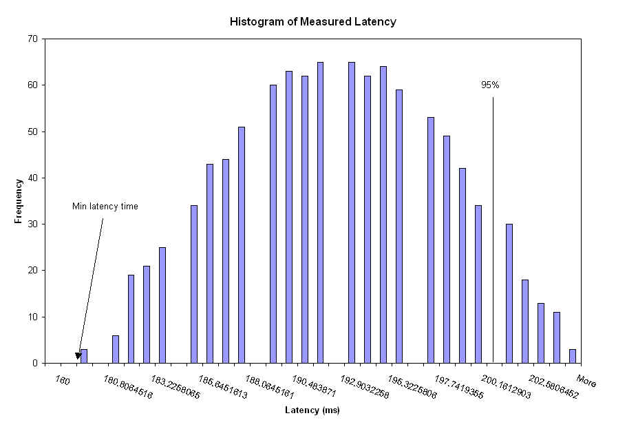
figure 3: actual measured latency histogram.
When a client requests data, we register the request with our Dynamic Latency module. The Dynamic Latency module then inspects the time based queue and measures the latency based on the current time and the time stamp of the packet at the head of the queue. The measured latency is accumulated, and after 100 measurements the dynamic latency module uses the low pass filter to adjust the latency.
It is important to realize that the 5% of packets that we don't receive in time do not result in data loss. The FEC allows us to determine the lost data.
Prior to a sample being shipped over the network, our Playout component encodes the packet with the required info to correctly reproduce the sample at the receiving end. During this step, we add the packet time stamp (synchronized to the next packet boundary) and information from previous samples to the FEC fields of the new packet. The Playout component stores a copy of the last packet sent across the network, thereby giving us access to the last three samples sent (the high, medium, and low quality versions within the stored packet). We discard the low quality version and resample the high and medium quality samples at half their previous sampling rate. To do this we create a new byte array of half the original size, and copy every other element of the original array into the new sample. We now combine these resampled versions of the previous two samples with the current sample (high quality) and send them across the network to the receiver.
At the receiving end the packet is decoded from the bytes received on the network into the Packet class format understood by our buffer and playout algorithms. When inserting the new packet into the buffer, we check to see whether either of the previous two packets were lost (see explanation in TimeBasedQueue). If so, we insert the redundant copies carried in the current packet. Each redundant sample is expanded to the original sample size by duplicating the degraded quality data. For the medium quality version each data point appears twice in the final sample, for the low quality version each data point is replicated four times as seen in figure 4.
figure 4: FEC sample results
We experimented with FEC quality by forcing the buffer to insert the redundant copies for each packet received. We ran a tests always using the medium quality version and tests always using the low quality version. The medium quality sample was very intelligible, with little distortion. The low quality sample added a significant amount of distortion and was much harder to comprehend. The .wav files from our tests appear below.
| Full Sample (wav) | Half Sample (wav) | Quarter Sample (wav) |
The time-based queue manages the receiving, ordering and storing of all packets into our Playout. When writing, we timestamp each packet with the current time of the sender rounded to the next packet boundary (based on the packet size set by the signaling team). The uniform packet size assures that each packet will arrive at the receiver timestamped on multiples of the packet size (packets with timestamp errors will be discarded). The time-based queue stores packets indexed by the synchronized packet timestamps. The first packet received sets the initial timestamp value, with each packet received afterwards inserted into the queue based on the multiples of the packet size between it and the head of the queue. For example if the packet size = 20ms, and the first entry in the queue has a timestamp of 60ms, a packet received with a timestamp of 80ms will be inserted in the second spot and a packet received with a timestamp of 120ms will be inserted in the fourth spot. Note that we never received a packet with a timestamp of 100ms. On receipt of the 120ms packet we insert a 'blank' packet into the third queue entry and use the redundant data contained in the 120ms packet to initialize the missed 100ms sample. If no redundant data exists (i.e. more than two blank packets need to be inserted), a packet initialized with constant silence in inserted into the missing position.
The queue has a separate buffer manager which periodically checks that entry at the head of the queue is current with the receiver's time stamp. Old packets (after considering network and read latency) are discarded from the queue. The architecture of our time-based queue also allows for integration of multiparty communication. Multiple packets received aligned on the same timestamp boundary are averaged together with those already in the queue. This allows for multiple users to synchronize their conversations into one playout packet.
The time server runs on the signal server and is started when the signal server is booted. The time server runs for the duration of the signal server's lifetime. When the server receives a request it stamps its current time in the request, and sends it back to the client. The time client determines the time at the server based on the measured network delay, and the response the server returned. This operation can be seen in figure 5 below.
figure 5: Operation of the time client/server system.
Server Time = t1 + (t2 - t0)
Time difference = Client Time - Server Time
Upon instantiation the time client object contacts the time server 6 times and determines the time difference. From the six time differences we remove the maximum and minimum values. The actual time difference we use is the average of the 4 remaining values.
The time client object provides a getTime() method which, based on the machines local time and the value of the time difference, will return the server time. Again, this relies on minimal clock drift. As explained above, getTime() is used to stamp all out going packets, and also used to determine when to play incoming packets.
We found that on the same subnet, synchronization is virtually undetectable (<1ms). In every test on different subnets the synchronization was less than 10ms.
We ran into problems in the exact semantics of our read and write functions. Particularly the Gateway required a different read model then that of our applications based on the restrictions of the dialogic card, and the our applications needed some way to synchronize and regulate their writing to the defined packetTime. To solve these problems we introduced non-blocking read for the Gateway, and a waitForWrite() function in the Connection interface.
The read method accessible through the Connection interface blocks waiting for data to be available at the head of the queue. Read blocks a variable amount of time based on the current dynamic latency, the read latency, and the current time of the receiver. This model, while correct for the needs of our applications, did not satisfy the restrictions imposed on the Gateway. The dialogic card requires that the Gateway be able to read data in chunks of 1024 bytes. Using the blocking read, the only possible way to satisfy this requirement would be by setting the packet size to this value. This would introduce a minimum of 128ms of latency not including the overhead due to processing and network delay. We solved this problem by allowing the Gateway to read without blocking. Thus for a packet size of 512 bytes (our current packet size) Gateway issues two data exchange reads for each dialogic request. If the data has not yet entered the buffer we return null to the Gateway. The non-blocking read was made accessible to the Gateway through a specific Gateway VoiceConnection interface.
When writing to a connection, we found that the applications had difficulty writing packets at packetTime intervals. We needed this synchronization in order to ensure the clients did not write more than one packet for each synchronized packet time block. We had two options, we could either make write block, or we could provide some method to allow the clients to tell when a previous write had finished (the packet time block had passed) and was ready for the next write. We chose the latter option as some applications may only write periodically and not desire the extra overhead imposed by blocking at each write. To provide this functionality we added a waitForWrite() method to our interface, which implements the second option by sleeping the time remaining in the packetTime interval.
Over the past months we’ve thoroughly researched the RTP specification and documentation. We’ve learned about the issues involved in designing a real time protocol, and the methods by which RTP attempts to address these problems (RTCP, etc…). We applied our learning from RTP to our implementations of Time Synchronization and the Time-Based Queue.
Over the course of the project we've learned about quality of service and the data-level methods to improve end-to-end QoS. As discussed above, we've attempted to reduce latency, jitter, and loss through adaptive playout, time-synchronized reading, and forward error correction. From the results of our experiments we've learned how to best adjust the latency parameters to minimize packet loss, how to insert redundant packets to compensate for last packets, and how to buffer packets to account for the burstiness of a connection. Our implementations described above represent our best effort at maximizing the QoS in the MIA project.
We've also learned about the work required behind integrating a multi-faceted project, and the additional requirements of this collaboration. In particular we've learned the necessity of communication, strictly defined interfaces, and responsibility for assigned tasks.
What we would do differently next time
We spent a significant amount of time researching methods to improve the performance of Java. In particular, we investigated the Java Native Interface (JNI) and the possiblity of moving our array modifying methods (for FEC and Packet averaging) to machine specific libraries. During this investigation we ran into many problems with the interface between Java and C, including the data type marshalling required for method calls through JNI (JNI did not correctly handle Java byte arrays). While this experience was educational, in the end we did not require the added performance given by the native calls. Surprisingly, Java's performance was more than sufficient for our needs. We could have saved ourselves time if we had structured the code in such a way to make native method substitutions viable, while at the same time leaving the actually performance tuning until we could evaluate the added benefit.
Similarly, it would have been more beneficial for MIA if we had produced a simple data shipping component before our more complex data exchange implementation. A simple socket-based implementation (not worrying about packet sizes, FEC, or time synchronization) might have allowed the other teams to begin testing earlier in the development cycle.
abstract public class DataExchange
// for signals
{
/**
* Opens a connection to host on
port. The Observer is used to handle all messages.
* This is used for non gateway
connections
**/
public static VoiceConnection
newConnection(CallBack observer,
InetAddress timeServerIP, Object params)
{
return
new ConnectionDX(observer, timeServerIP, params );
}
/**
* Opens a connection to host on
port. The Observer is used to handle all messages.
* This is used for the gateway
only.
**/
public static VoiceConnection
newConnectionGateway(CallBack observer,
InetAddress timeServerIP, Object params)
{
return
new ConnectionGatewayDX(observer, timeServerIP, params );
}
}
/**
* The connection interface is used by signals and
* provides access to the connection.
**/
public interface VoiceConnection // for signals
{
public byte[] read();
// read samples
public void write(byte [] s);
// write samples
public void waitForWrite();
// wait for last write to finish
public void close();
// shuts down the connection
public void open();
// starts the connection
public int getOptimalWriteSize();
// the optimal size to write.
public void setParams(
CMS_MsgDataXParams params);
// update management parameters
public ConnectionTable getConnectionTable();
// handle to the connection table
public String toString();
}
/**
* The connection table specifies hosts involved in
the call
* Out going packets will be sent to everyone in the
connection table
* incomming packets will be accepted if host is in
the table
**/
public interface ConnectionTable extends Enumeration
// for signals
{
public static final int MAX_CONNECTIONS
= 16;
public void add(InetAddress hostAddress,
int hostPort);
public void delete(InetAddress
hostAddress, int hostPort);
public boolean isMember(InetAddress
hostAddress, int hostPort);
public Enumeration connections();
public boolean connectionsExist();
int getMyPort();
byte getUniqueID(InetAddress hostAddress,
int hostPort);
}
/**
* The CallBack's are used to signify noteable data
exchange events
**/
public interface CallBack
// for signals
{
public void handleEvent(int event);
}
Our resources were limited throughout the course. For many of the puzzles babbage was overloaded. Also for the project, because we generally needed at least two computers to test, the one machine provided was insufficient. Christi was always 15 mintues late to lecture -- is this acceptable?
RTP: http://www.cs.columbia.edu/~hgs/rtp/
Java: Inside Java, Java in a Nutshell
Spoons
This page was last modified 01/01/02 06:41 PM