Computational Graphs

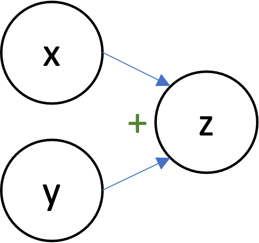
- Each node represents an scalar/vector/tensor/array.
- Edges represent dependencies.
- $y \rightarrow u$ means that $y$ was used to compute $u$
In Python, we can use operator overloading and dynamic typing. Suppose I write a function
def f(x):
    return x*x + 1.0
imagining that we will call it with x being a floating-point number.
x being a dual number (because Python is not explicitly typed). * and + desugar to calls to my __mul__ and __add__ methods.Problem: can't just compute derivatives as-we-go like with forward mode AD.
Same as before: we replace each number/array $y$ with a pair, except this time the pair is not $(y, \frac{\partial y}{\partial x})$ but instead $(y, \nabla_y \ell)$ where $\ell$ is one fixed output.
Suppose that the output $\ell$ can be written as $$\ell = f(u), \; u = g(y).$$ Here, $g$ represents the immediate next operation that consumes the intermediate value $y$ (producing a new intermediate $u$), and $f$ represents all the rest of the computation. Suppose all these expressions are scalars. By the chain rule, $$\frac{\partial \ell}{\partial y} = g'(y) \cdot \frac{\partial \ell}{\partial u}.$$ That is, we can compute $\frac{\partial \ell}{\partial y}$ using only "local" information (information that's available in the program around where $y$ is computed and used) and $\frac{\partial \ell}{\partial u}$.
More generally, suppose that the output $\ell$ can be written as $$\ell = F(u_1, u_2, \ldots, u_k), \; u_i = g_i(y).$$ Here, the $g_1, g_2, \ldots, g_k$ represent the immediate next operations that consume the intermediate value $y$ (note that there may be many such $g$), the $u_i$ are the arrays output by those operations, and $F$ represents all the rest of the computation. By the multivariate chain rule, $$\nabla_y \ell = \sum_{i=1}^k D g_i(y)^T \nabla_{u_i} \ell.$$ Again, we see that we can compute $\frac{\partial \ell}{\partial y}$ using only "local" information and the gradients of the loss with respect to each array that immediately depends on $y$, i.e. $\nabla_{u_i} \ell$.
Idea: remember the order in which we computed all the intermediate arrays/tensors, and then compute their gradients in the reverse order.
High-level BP algorithm:
Suppose $u \in \mathbb{R}^n$ and $y \in \mathbb{R}^m$. Then $D_y u \in \mathbb{R}^{n \times m}$ and $(D_y u)^T \in \mathbb{R}^{m \times n}$. And note that $\nabla_{u} \ell \in \mathbb{R}^n$

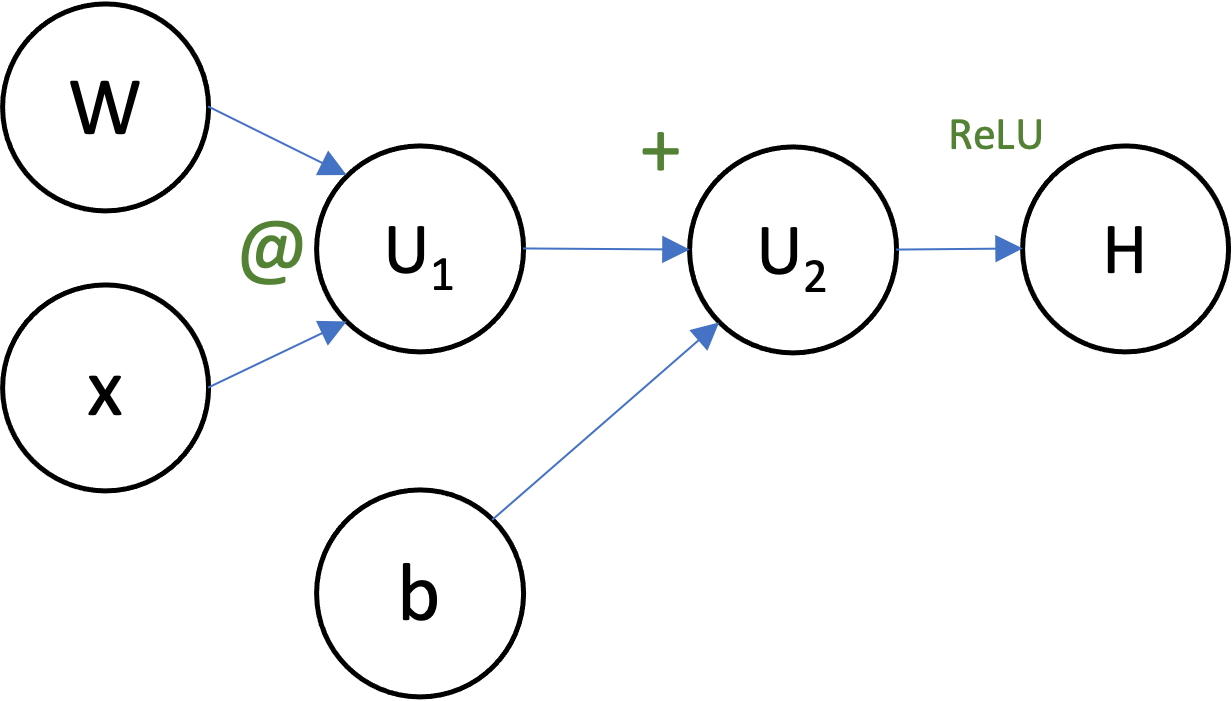
Can you draw the computational graph for the function
$$H = \max(0, Wx+b)$$for $W \in \mathbb{R}^{c \times d}$, $x \in \mathbb{R}^d$, and $b \in \mathbb{R}^c$?

To do backprop in a computation represented by a computational graph:
Using your computational graph, suppose that $W = 2$, $x = 3$, and $b = 1$. Write out (in order!) the steps that backprop would to to compute the gradients of $H$ with respect to everything ($W$, $x$, and $b$).

Note: $17 \cdot 18 = 306$ (according to ChatGPT)
Advantages:
Disadvantages: