Estimating Probabilities from data

Remember the Bayes Optimal classifier: If we are provided with $P(X,Y)$ we can predict the most likely label for $\mathbf{x}$, formally ${\mathrm{argmax}}_{y}P(y|\mathbf{x})$. It is therefore worth considering if we can estimate $P(X,Y)$ directly from the training data. If this is possible (to a good approximation) we could then use the Bayes Optimal classifier in practice on our estimate of $P(X,Y)$.

In fact, many supervised learning can be viewed as estimating $P(X,Y)$. Generally, they fall into two categories:

• When we estimate $P(X,Y)=P(X|Y)P(Y)$, then we call it generative learning.
• When we only estimate $P(Y|X)$ directly, then we call it discriminative learning.

Simple scenario: coin toss

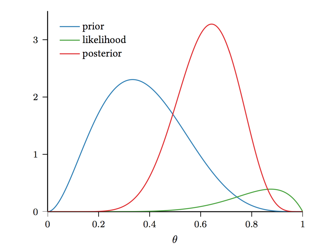
Suppose you find a coin and it's ancient and very valuable. Naturally, you ask yourself, "What is the probability that this coin comes up heads when I toss it?" You toss it $n=10$ times and obtain the following sequence of outcomes: $D=\{H,T,T,H,H,H,T,T,T,T\}$. Based on these samples, how would you estimate $P(H)$? We observed $n_H=4$ heads and $n_T=6$ tails. So, intuitively, $$P(H)\approx \frac{n_H}{n_H+n_T}=\frac{4}{10}=0.4$$ Can we derive this more formally?

Maximum Likelihood Estimation (MLE)

The estimator we just mentioned is the Maximum Likelihood Estimate (MLE). For MLE you typically proceed in two steps: First, you make an explicit modeling assumption about what type of distribution your data was sampled from. Second, you set the parameters of this distribution so that the data you observed is as likely as possible.

Let us return to the coin example. A natural assumption about a coin toss is that the distribution of the observed outcomes is a binomial distribution. The binomial distribution has two parameters $n$ and $\theta$ and it captures the distribution of $n$ independent Bernoulli (i.e. binary) random events that have a positive outcome with probability $\theta$. In our case $n$ is the number of coin tosses, and $\theta$ could be the probability of the coin coming up heads (e.g. $P(H)=\theta$). Formally, the binomial distribution is defined as $$\begin{array}{rl}P(D\mid \theta )& =\left(\begin{array}{c}{n}_H+n_T\\ n_H\end{array}\right){\theta }^{n_H}(1-\theta {)}^{n_T},\end{array}$$ and it computes the probability that we would observe exactly $n_H$ heads, $n_T$ tails, if a coin was tossed $n=n_H+n_T$ times and its probability of coming up heads is $\theta$.

MLE Principle: Find $\hat{\theta }$ to maximize the likelihood of the data, $P(D;\theta )$: $$\begin{array}{rl}{\hat{\theta }}_{MLE}& =\underset{\theta }{\mathrm{argmax}}P(D;\theta )\end{array}$$

Often we can solve this maximization problem with a simple two step procedure: 1. plug in all the terms for the distribution, and take the $\log$ of the function. 2. Compute its derivative, and equate it with zero. Taking the log of the likelihood (often referred to as the log-likelihood) does not change its maximum (as the log is a monotonic function, and the likelihood positive), but it turns all products into sums which are much easier to deal with when you differentiate. Equating the derivative with zero is a standard way to find an extreme point. (To be precise you should verify that it really is a maximum and not a minimum, by verifying that the second derivative is negative.)

Returning to our binomial distribution, we can now plug in the definition and compute the log-likelihood: $$\begin{array}{rl}{\hat{\theta }}_{MLE}& =\underset{\theta }{\mathrm{argmax}}P(D;\theta )\\ & =\underset{\theta }{\mathrm{argmax}}\left(\begin{array}{c}{n}_H+n_T\\ n_H\end{array}\right){\theta }^{n_H}(1-\theta {)}^{n_T}\\ & =\underset{\theta }{\mathrm{argmax}}\log \left(\begin{array}{c}{n}_H+n_T\\ n_H\end{array}\right)+n_H\cdot \log (\theta )+n_T\cdot \log (1-\theta )\\ & =\underset{\theta }{\mathrm{argmax}}{n}_H\cdot \log (\theta )+n_T\cdot \log (1-\theta )\end{array}$$ We can then solve for $\theta$ by taking the derivative and equating it with zero. This results in $$\begin{array}{r}\frac{n_H}{\theta }=\frac{n_T}{1-\theta }⟹n_H-n_H\theta =n_T\theta ⟹\theta =\frac{n_H}{n_H+n_T}\end{array}$$ A nice sanity check is that $\theta \in [0,1]$.

• MLE gives the explanation of the data you observed.
• If $n$ is large and your model/distribution is correct (that is $\mathcal{H}$ includes the true model), then MLE finds the true parameters.
• But the MLE can overfit the data if $n$ is small. It works well when $n$ is large.
• If you do not have the correct model (and $n$ is small) then MLE can be terribly wrong!

Simple scenario: coin toss with prior knowledge

Assume you have a hunch that $\theta$ is close to $0.5$. But your sample size is small, so you don't trust your estimate. Simple fix: Add $m$ imaginery throws that would result in ${\theta }^{\prime }$ (e.g. $\theta =0.5$). Add $m$ Heads and $m$ Tails to your data. $$\hat{\theta }=\frac{n_H+m}{n_H+n_T+2m}$$ For large $n$, this is an insignificant change. For small $n$, it incorporates your "prior belief" about what $\theta$ should be. Can we derive this formally?

The Bayesian Way

Model $\theta$ as a random variable, drawn from a distribution $P(\theta )$. Note that $\theta$ is not a random variable associated with an event in a sample space. In frequentist statistics, this is forbidden. In Bayesian statistics, this is allowed and you can specify a prior belief $P(\theta )$ defining what values you believe $\theta$ is likely to take on.

Now, we can look at $P(\theta \mid D)=\frac{P(D\mid \theta )P(\theta )}{P(D)}$ (recall Bayes Rule!), where

• $P(\theta )$ is the prior distribution over the parameter(s) $\theta$, before we see any data.
• $P(D\mid \theta )$ is the likelihood of the data given the parameter(s) $\theta$.
• $P(\theta \mid D)$ is the posterior distribution over the parameter(s) $\theta$ after we have observed the data.

A natural choice for the prior $P(\theta$) is the Beta distribution: $$\begin{array}{r}P(\theta )=\frac{{\theta }^{\alpha -1}(1-\theta {)}^{\beta -1}}{B(\alpha ,\beta )}\end{array}$$ where $B(\alpha ,\beta )=\frac{\mathrm{\Gamma }(\alpha )\mathrm{\Gamma }(\beta )}{\mathrm{\Gamma }(\alpha +\beta )}$ is the normalization constant (if this looks scary don't worry about it, it is just there to make sure everything sums to $1$ and to scare children at Halloween). Note that here we only need a distribution over a single binary random variable $\theta$. (The multivariate generalization of the Beta distribution is the Dirichlet distribution.)

Why is the Beta distribution a good fit?

• it models probabilities ($\theta$ lives on $[0,1]$)
• it is of the same distributional family as the binomial distribution (conjugate prior) $\to$ the math will turn out nicely:

So far, we have a distribution over $\theta$. How can we get an estimate for $\theta$?

Maximum a Posteriori Probability Estimation (MAP)

A few comments:

• The MAP estimate is identical to MLE with $\alpha -1$ hallucinated heads and $\beta -1$ hallucinated tails
• As $n\to \mathrm{\infty }$, ${\hat{\theta }}_{MAP}\to {\hat{\theta }}_{MLE}$ as $\alpha -1$ and $\beta -1$ become irrelevant compared to very large $n_H,n_T$.
• MAP is a great estimator if an accurate prior belief is available (and mathematically tractable).
• If $n$ is small, MAP can be very wrong if prior belief is wrong!

"True" Bayesian approach

Note that MAP is only one way to get an estimator. There is much more information in $P(\theta \mid D)$, and it seems like a shame to simply compute the mode and throw away all other information. A true Bayesian approach is to use the posterior predictive distribution directly to make prediction about the label $Y$ of a test sample with features $X$: $$P(Y\mid D,X)={\int }_{\theta }P(Y,\theta \mid D,X)d\theta ={\int }_{\theta }P(Y\mid \theta ,D,X)P(\theta |D)d\theta$$ Unfortunately, the above is generally intractable in closed form and sampling techniques, such as Monte Carlo approximations, are used to approximate the distribution. A pleasant exception are Gaussian Processes, which we will cover later in this course.

Another exception is actually our coin toss example. To make predictions using $\theta$ in our coin tossing example, we can use $$\begin{array}{rl}P(heads\mid D)=& {\int }_{\theta }P(heads,\theta \mid D)d\theta \\ =& {\int }_{\theta }P(heads\mid \theta ,D)P(\theta \mid D)d\theta \text{(Chain rule: }P(A,B|C)=P(A|B,C)P(B|C)\text{.)}\\ =& {\int }_{\theta }\theta P(\theta \mid D)d\theta \\ =& E[\theta |D]\\ =& \frac{n_H+\alpha }{n_H+\alpha +n_T+\beta }\end{array}$$ Here, we used the fact that we defined $P(heads\mid D,\theta )=P(heads\mid \theta )=\theta$ (this is only the case because we assumed that our data is drawn from a binomial distribution - in general this would not hold).

Machine Learning and estimation

• MLE Prediction: $P(y|x_t;\theta )$ Learning: $\theta ={\mathrm{argmax}}_{\theta }P(D;\theta )$. Here $\theta$ is purely a model parameter.
• MAP Prediction: $P(y|x_t,\theta )$ Learning: $\theta ={\mathrm{argmax}}_{\theta }P(\theta |D)\propto P(D\mid \theta )P(\theta )$. Here $\theta$ is a random variable.
• "True Bayesian" Prediction: $P(y|x_t,D)={\int }_{\theta }P(y|\theta )P(\theta |D)d\theta$. Here $\theta$ is integrated out - our prediction takes all possible models into account.

As always the differences are subtle. In MLE we maximize $\log [P(D;\theta )]$ in MAP we maximize $\log [P(D|\theta )]+\log [P(\theta )]$. So essentially in MAP we only add the term $\log [P(\theta )]$ to our optimization. This term is independent of the data and penalizes if the parameters, $\theta$ deviate too much from what we believe is reasonable. We will later revisit this as a form of regularization, where $\log [P(\theta )]$ will be interpreted as a measure of classifier complexity.