| Loss | Usage | Comments |
|---|
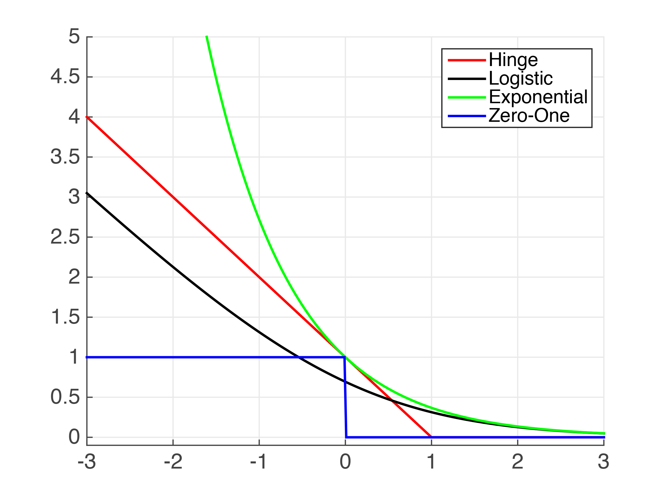
| Hinge-Loss |
Standard SVM()(Differentiable) Squared Hingeless SVM () | When used for Standard SVM, the loss function denotes the size of the margin between linear separator and its closest points in either class. Only differentiable everywhere with . |
| Log-Loss | Logistic Regression | One of the most popular loss functions in Machine Learning, since its outputs are well-calibrated probabilities. |
| Exponential Loss | AdaBoost | This function is very aggressive. The loss of a mis-prediction increases exponentially with the value of . This can lead to nice convergence results, for example in the case of Adaboost, but it can also cause problems with noisy data. |
| Zero-One Loss | Actual Classification Loss | Non-continuous and thus impractical to optimize. |