10: Empirical Risk Minimization

Loading [MathJax]/jax/output/HTML-CSS/fonts/TeX/fontdata.js

10: Empirical Risk Minimization

Recap

Remember the unconstrained SVM Formulation

$\min_{\mathbf{w}}\ C\underset{Hinge-Loss}{\underbrace{\sum_{i=1}^{n}\max[1-y_{i}\underset{h({\mathbf{x}_i})}{\underbrace{(w^{\top}{\mathbf{x}_i}+b)}},0]}}+\underset{l_{2}-Regularizer}{\underbrace{\left\Vert w\right\Vert _{z}^{2}}}$ The hinge loss is the SVM's error function of choice, whereas the

$\left.l_{2}\right.$ -regularizer reflects the complexity of the solution, and penalizes complex solutions. This is an example of empirical risk minimization with a loss function

$\ell$ and a regularizer

$r$ ,

$\min_{\mathbf{w}}\frac{1}{n}\sum_{i=1}^{n}\underset{Loss}{\underbrace{l(h_{\mathbf{w}}({\mathbf{x}_i}),y_{i})}}+\underset{Regularizer}{\underbrace{\lambda r(w)}},$ where the loss function is a continuous function which penalizes training error, and the regularizer is a continuous function which penalizes classifier complexity. Here, we define

$\lambda$ as

$\frac{1}{C}$ from the previous lecture.^[1]

Commonly Used Binary Classification Loss Functions

Different Machine Learning algorithms use different loss functions; Table 4.1 shows just a few:

Loss $\ell(h_{\mathbf{w}}(\mathbf{x}_i,y_i))$	Usage	Comments
Hinge-Loss $\max\left[1-h_{\mathbf{w}}(\mathbf{x}_{i})y_{i},0\right]^{p}$	Standard SVM( $\left.p=1\right.$ ) (Differentiable) Squared Hingeless SVM ( $\left.p=2\right.$ )	When used for Standard SVM, the loss function denotes the size of the margin between linear separator and its closest points in either class. Only differentiable everywhere with $\left.p=2\right.$ .
Log-Loss $\left.\log(1+e^{-h_{\mathbf{w}}(\mathbf{x}_{i})y_{i}})\right.$	Logistic Regression	One of the most popular loss functions in Machine Learning, since its outputs are well-calibrated probabilities.
Exponential Loss $\left. e^{-h_{\mathbf{w}}(\mathbf{x}_{i})y_{i}}\right.$	AdaBoost	This function is very aggressive. The loss of a mis-prediction increases exponentially with the value of $-h_{\mathbf{w}}(\mathbf{x}_i)y_i$ . This can lead to nice convergence results, for example in the case of Adaboost, but it can also cause problems with noisy data.
Zero-One Loss $\left.\delta(\textrm{sign}(h_{\mathbf{w}}(\mathbf{x}_{i}))\neq y_{i})\right.$	Actual Classification Loss	Non-continuous and thus impractical to optimize.

Table 4.1: Loss Functions With Classification

$\left.y\in\{-1,+1\}\right.$

Quiz: What do all these loss functions look like with respect to

$\left.z=yh(\mathbf{x})\right.$ ?

Figure 4.1: Plots of Common Classification Loss Functions - x-axis: $\left.h(\mathbf{x}_{i})y_{i}\right.$ , or "correctness" of prediction; y-axis: loss value

Some questions about the loss functions:

Which functions are strict upper bounds on the 0/1-loss?
What can you say about the hinge-loss and the log-loss as $\left.z\rightarrow-\infty\right.$ ?

Commonly Used Regression Loss Functions

Loss $\ell(h_{\mathbf{w}}(\mathbf{x}_i,y_i))$						Comments
Squared Loss $\left.(h(\mathbf{x}_{i})-y_{i})^{2}\right.$						Most popular regression loss function Estimates Mean Label ADVANTAGE: Differentiable everywhere DISADVANTAGE: Somewhat sensitive to outliers/noise Also known as Ordinary Least Squares (OLS)
Absolute Loss $\left.\|h(\mathbf{x}_{i})-y_{i}\|\right.$						Also a very popular loss function Estimates Median Label ADVANTAGE: Less sensitive to noise DISADVANTAGE: Not differentiable at $0$
Huber Loss $\left.\frac{1}{2}\left(h(\mathbf{x}_{i})-y_{i}\right)^{2}\right.$ if $\|h(\mathbf{x}_{i})-y_{i}\|<\delta$ , otherwise $\left.\delta(\|h(\mathbf{x}_{i})-y_{i}\|-\frac{\delta}{2})\right.$						Also known as Smooth Absolute Loss ADVANTAGE: "Best of Both Worlds" of Squared and Absolute Loss Once-differentiable Takes on behavior of Squared-Loss when loss is small, and Absolute Loss when loss is large.
Log-Cosh Loss $\left.log(cosh(h(\mathbf{x}_{i})-y_{i}))\right.$ , $\left.cosh(x)=\frac{e^{x}+e^{-x}}{2}\right.$						ADVANTAGE: Similar to Huber Loss, but twice differentiable everywhere

Table 4.2: Loss Functions With Regression, i.e.

$\left.y\in\mathbb{R}\right.$

Quiz:

$\left.z=h(\mathbf{x}_{i})-y_{i}\right.$

Figure 4.2: Plots of Common Regression Loss Functions - x-axis: $\left.h(\mathbf{x}_{i})y_{i}\right.$ , or "error" of prediction; y-axis: loss value

Regularizers

$\begin{equation} \min_{\mathbf{w},b} \sum_{i=1}^n\ell(h_\mathbf{w}(\mathbf{x}),y_i)+\lambda r(\mathbf{w}) \Leftrightarrow \min_{\mathbf{w},b} \sum_{i=1}^n\ell(h_\mathbf{w}(\mathbf{x}),y_i) \textrm { subject to: } r(\mathbf{w})\leq B \end{equation}$

$\left.\lambda\geq0\right.$

$\left.B\geq0\right.$

$\left.l_{2}\right.$

Regularizer $r(\mathbf{w})$						Properties
$l_{2}$ -Regularization $\left.r(\mathbf{w}) = \mathbf{w}^{\top}\mathbf{w} = \\|{\mathbf{w}}\\|_{2}^{2}\right.$						ADVANTAGE: Strictly Convex ADVANTAGE: Differentiable DISADVANTAGE: Uses weights on all features, i.e. relies on all features to some degree (ideally we would like to avoid this) - these are known as Dense Solutions.
$l_{1}$ -Regularization $\left.r(\mathbf{w}) = \\|\mathbf{w}\\|_{1}\right.$						Convex (but not strictly) DISADVANTAGE: Not differentiable at $0$ (the point which minimization is intended to bring us to Effect: Sparse (i.e. not Dense) Solutions
Elastic Net $\left.\alpha\\|\mathbf{w}\\|_{1}+(1-\alpha)\\|{\mathbf{w}}\\|_{2}^{2}\right.$ $\left.\alpha\in[0, 1)\right.$						ADVANTAGE: Strictly convex (i.e. unique solution) DISADVANTAGE: Non-differentiable
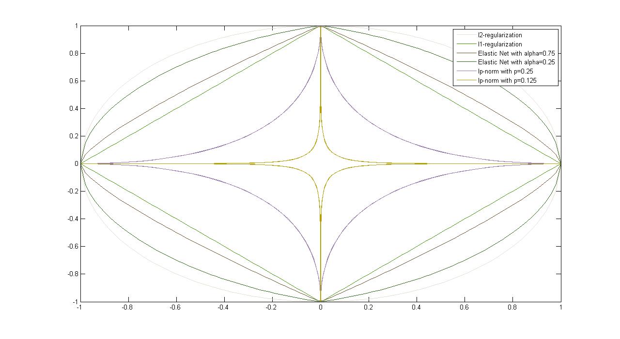
$l_p$ -Norm $\left.\\|{\mathbf{w}}\\|_{p} = (\sum\limits_{i=1}^d v_{i}^{p})^{1/p}\right.$						(often $\left.0<p\leq1\right.$ ) DISADVANTAGE: Non-convex ADVANTAGE: Very sparse solutions Initialization dependent DISADVANTAGE: Not differentiable

Table 4.3: Types of Regularizers

Figure 4.3: Plots of Common Regularizers

Famous Special Cases

Loss and Regularizer						Comments
Ordinary Least Squares $\min_{\mathbf{w}} \frac{1}{n}\sum\limits_{i=1}^n (\mathbf{w}^{\top}x_{i}-y_{i})^{2}$						Squared Loss No Regularization Closed form solution: $\left.\mathbf{w}=(\mathbf{X}\mathbf{X}^\top)^{-1}\mathbf{X}\mathbf{y}^{\top}\right.$ $\left.\mathbf{X}=[\mathbf{x}_{1}, ..., \mathbf{x}_{n}]\right.$ $\left.\mathbf{y}=[y_{1},...,y_{n}]\right.$
Ridge Regression $\min_{\mathbf{w}} \frac{1}{n}\sum\limits_{i=1}^n (\mathbf{w}^{\top}x_{i}-y_{i})^{2}+\lambda\\|{w}\\|_{2}^{2}$						Squared Loss $l_{2}$ -Regularization $\left.\mathbf{w}=(\mathbf{X}\mathbf{X}^{\top}+\lambda\mathbb{I})^{-1}\mathbf{X}\mathbf{y}^{\top}\right.$
Lasso $\min_{\mathbf{w}} \frac{1}{n}\sum\limits_{i=1}^n (\mathbf{w}^{\top}\mathbf{x}_{i}-{y}_{i})^{2}+\lambda\\|\mathbf{w}\\|_{1}$						+ sparsity inducing (good for feature selection) + Convex - Not strictly convex (no unique solution) - Not differentiable (at 0) Solve with (sub)-gradient descent or SVEN
Logistic Regression $\min_{\mathbf{w},b} \frac{1}{n}\sum\limits_{i=1}^n \log{(1+e^{-y_i(\mathbf{w}^{\top}\mathbf{x}_{i}+b)})}$						Often $l_{1}$ or $l_{2}$ Regularized Solve with gradient descent. $\left.\Pr{(y\|x)}=\frac{1}{1+e^{-y(\mathbf{w}^{\top}x+b)}}\right.$
Linear Support Vector Machine $\min_{\mathbf{w},b} C\sum\limits_{i=1}^n \max[1-y_{i}\mathbf{w}^\top{\mathbf{x}_i})]+\\|\mathbf{w}\\|_2^2$						Typically $l_2$ regularized (sometimes $l_1$ ). Quadratic program. When kernelized leads to sparse solutions. Kernelized version can be solved very efficiently with specialized algorithms (e.g. SMO)

Table 4.4: Special Cases

Ridge Regression is very fast if data isn't too high dimensional.
Ridge Regression is just 1 line of Julia / Python.
There is an interesting connection between Ordinary Least Squares and the first principal component of PCA (Principal Component Analysis). PCA also minimizes square loss, but looks at perpendicular loss (the horizontal distance between each point and the regression line) instead.

[1] In Bayesian Machine Learning, it is common to optimize

$\lambda$ , but for the purposes of this class, it is assumed to be fixed.