AutoStitch

CS 5670 Introduction to Computer Vision

Brian Orecchio and Kevin Green

Major Design Choices

To warp an image to spherical coordinates, we did not do anything different than what the typical approach is.

To align the images, we first used the RANSAC algorithm to find the homography/translation that best fit the matches that were given by the feature matching. The number of iterations is an input so all we had to do for each iteration is to pick a random number of matches for the model we are using (1 match for a translation and 4 for a homography), then compute the transformation that is the mapping between the matches. Then we just use this transformation as the mapping between all the other matches and count the inliers. After all the iterations have been completed, we use the maximunm number of inliers plus the matches that produced the transformation to compute a final transfomation using least squares. The least squares solution was obtained for the homography model by doing an SVD on the matrix A which gives us the solution as the last column of the matrix V since we want the the eigenvector of A^TA corresponding to the smallest eigenvalue. The solution for the translation model was obtained by finding the average translation between all the matches.

To do the blending operation, we used the inverse of the transformation that is computed when aligning the images to do the inverse mapping between our accumulated image and the image that is being added. This means that we looped over the possible pixels in accumulated image and for each pixel, found if it appears somewhere in the new image based on the inverse transformation. If it is found in the new image, we used the PixelLerp function to interpolate the color value at that pixel and this color becomes the color of the pixel in the accumulated image. To do the actual blending, we used a linear feathering technique where we weight the values around some specified border of the image less and less as the border is approached. We also had to normalize the blending by keeping track of the alpha values for each pixel as we go and dividing by alpha at the end. The only other design choice that was made was how to correct the drift of a 360 panorama. We fixed this drift by finding out how much the y value of a certain pixel in the first and last images differs and sheared the image in the y direction by the difference divided by the width of the accumulated image.

There were some things that worked well and things that didn't. At first we blended the images based on how close the pixel is to the left and right border along with the top and bottom. This didn't work as well as just blending based on the horizontal position which is what we used in our final code. We also started off looping over the entire accumulated image in the blending routine but realized that we only need to loop over 'candidate pixels'. We noticed that creating a panorama with spherical warping and translations worked better than a homography when large panoramas were desired. For the blending, the feathering worked pretty well except when there was large overall differences in the brightness of two adjacent images. There was still a smooth blend in that case but the results still looked slightly non-continuous.

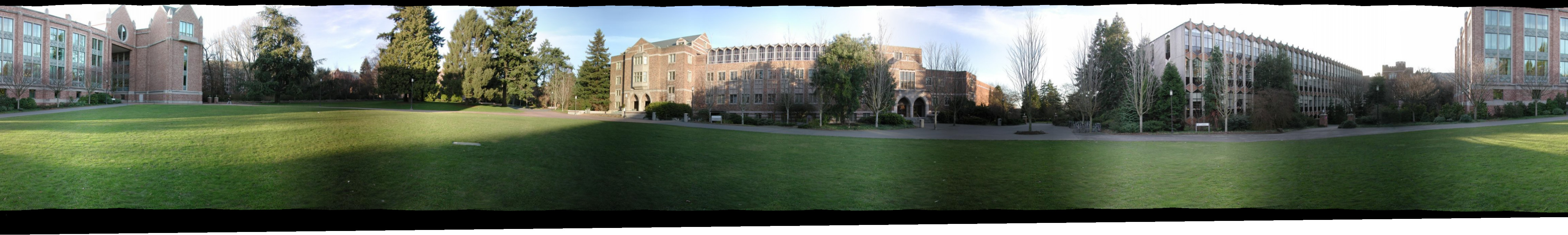
360 Panoramas

Test Panorama

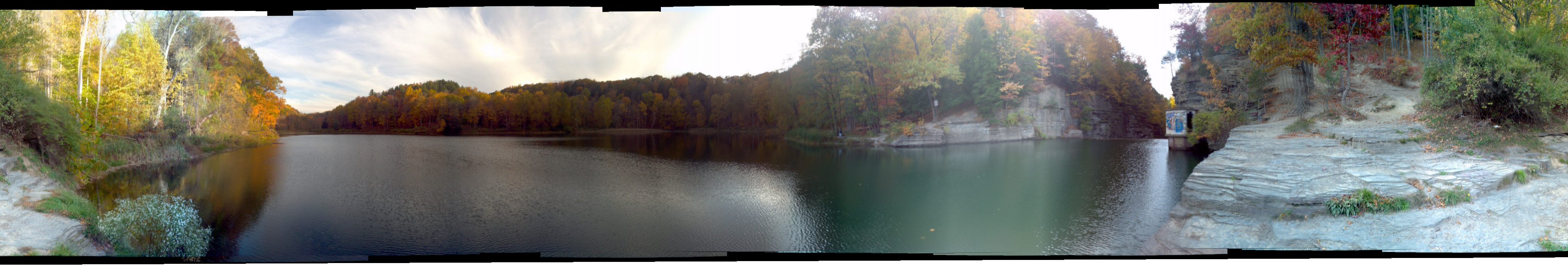Panorama taken at a popular spot in Ithaca where people go gorge jumping.

Panoramas created by Homographies

Panorama created with 3 test images using the homography method.

Panorama created with 5 test images using the homography method. We can see that the method is breaking down since our viewing angle is so large. Due to perspective projection, when we have too big of a field of view for the panorama, the warping needed to align the matched points is too distorted to create a good mosaic image. This does not happen when were are creating a 360 panorama after spherically warping the images since the transformations between the warped images are just affine translations and not homographies. This homography method of creating panoramas will break down at different rates depending on the images used.

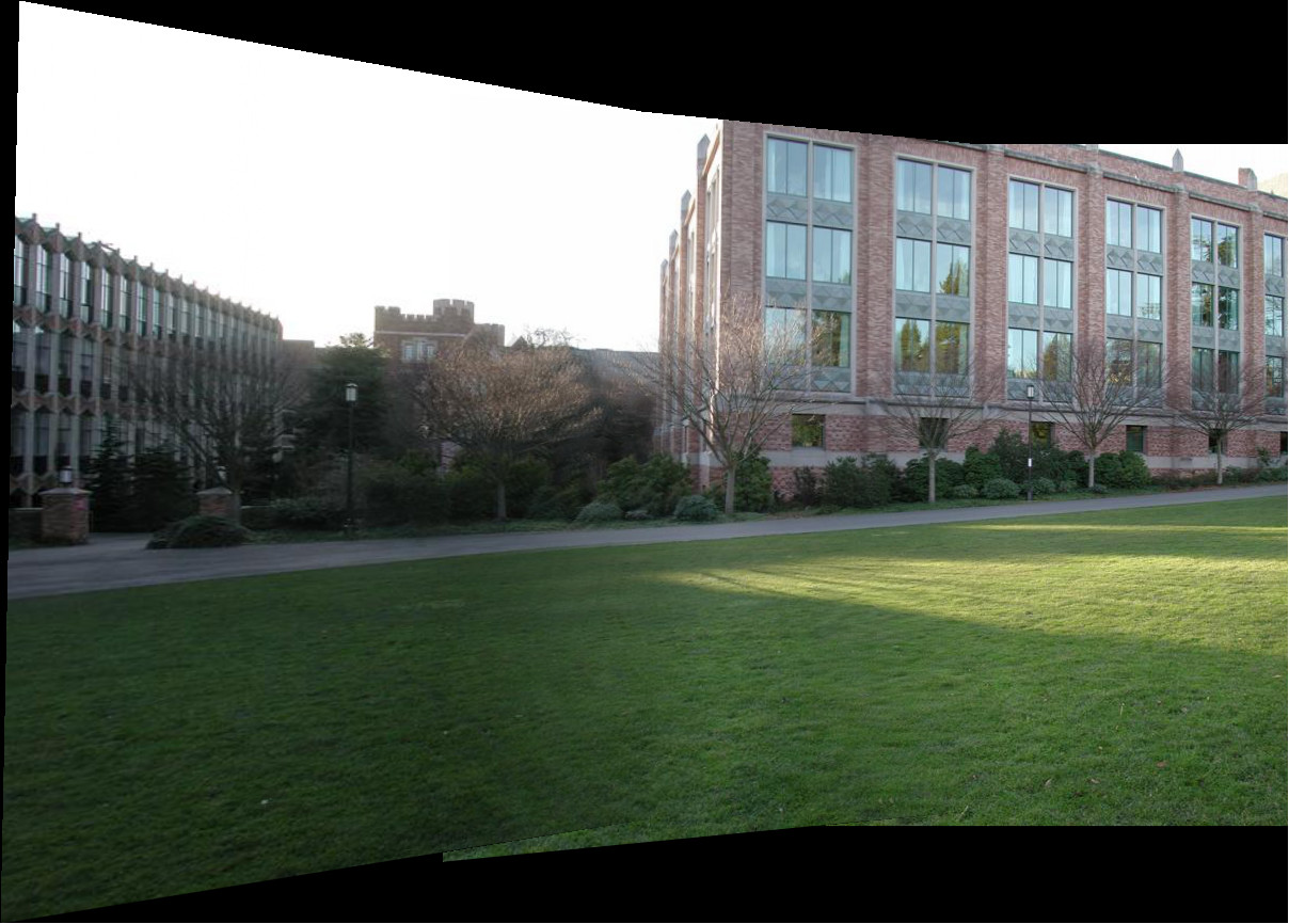
Panorama created with 2 images from the gorge jumping spot using the homography method.

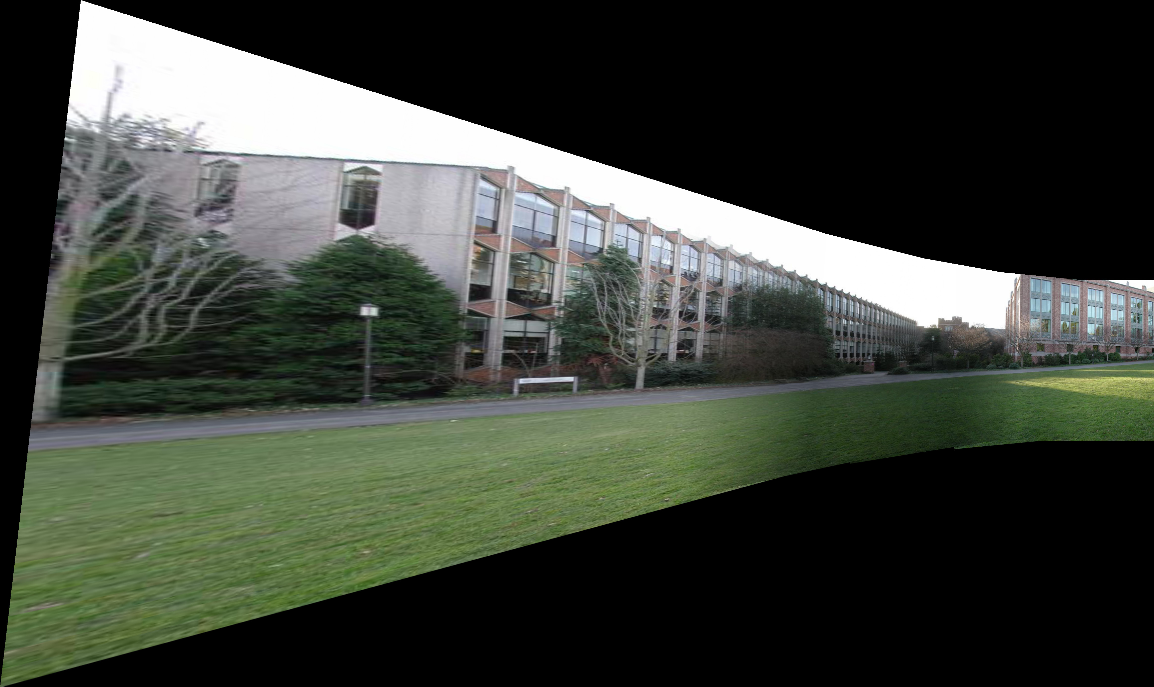
Panorama created with 3 images from the gorge jumping spot using the homography method. We can start to see this method breaking down.