I. Design

Feature Detection

Feature detection was performed by computing Harris values c(H) using 2x2 weighted Harris matrices H. To provide invariance to rotation, a 5x5 Gaussian mask was used to assign weights to each Harris matrix using neighboring pixels. For computational efficiency, Harris values were estimated using the determinant and trace values of the Harris matrix. When selecting specific pixel locations to represent features, a simple dynamic thresholding method was used to select an appropriate Harris value threshold. The mean (µ) and standard deviation (σ) of Harris values were calculated across the image. Assuming the values follow a roughly Gaussian distribution, an initial threshold of µ + 2σ, which results in detecting approximately 2.2% of the pixels as features.

Figure 1. Gaussian Distribution
(http://en.wikipedia.org/wiki/Normal_distribution)

Using this initial thresholding value, local maxima were identified in a 5x5 window and used as feature locations. If the number of detected features is less than the MIN_FEATURES constant parameter, then the dynamic method incrementally decreases the threshold until this condition is met.

The pixel location and angle is specified for each detected feature. To determine the angle or orientation of the feature, a 7x7 Gaussian kernel was used to apply a low-pass filter. The filter is used to reduce noise in the image that could drastically change the gradient at a single location. After pre-filtering, 3x3 sobel filters were applied to obtain the gradients in the x and y direction. The angle is then calculated by taking the arctangent of the y-grad divided by the x-grad.

Feature Description

Two feature descriptors were implemented: (1) a simple 5x5 square window descriptor (without orientation) and (2) a simplified MOPS descriptor. In the previous feature detection stage, pixel locations within 20 pixels of the image boundary are ignored and not used as features. This prevents descriptors from having varying lengths, which would otherwise cause issues during matching.

The simplified MOPS descriptor sub-samples 8x8 patches from a 41x41 pixel region around the feature using a low-passed image (7x7 Gaussian kernel). Low-pass filtering the image prior to sub-sampling prevents aliasing in the reduced image. The 8x8 patch is oriented by using the inverse matrix of the rotation transform and applying bilinear interpolation to estimate the correct pixel value of the rotated point.

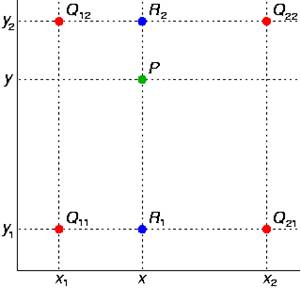
Figure 2. Bilinear Interpolation
(http://en.wikipedia.org/wiki/Bilinear_interpolation)

*Note: The rotation is applied after centering the origin on the feature location. After rotation and interpolation, the 8x8 patch is normalized to have a zero mean and unit variance. The normalization provides invariance to affine intensity changes.

Feature Matching

The “ratio test” was implemented as the matching score, where the score is equal to the distance of the current feature to the best feature in the second image divided by the distance of the current feature to the second best feature in the other image. This ratio is between 0 and 1, where 0 indicates a strong match and 1 indicates an ambiguous match.

I. Evaluation

Plots

Figure 3. “Graf” Results

“Graf” AUC Summary

Descriptor/Matching Method	Area Under Curve
Simple + SSD	0.673416
Simple + Ratio Test	0.708075
MOPS + SSD	0.900277
MOPS + Ratio Test	0.928643

Figure 4. “Yosemite” Results

“Yosemite” AUC Summary

Descriptor/Matching Method	Area Under Curve
Simple + SSD	0.902653
Simple + Ratio Test	0.888056
MOPS + SSD	0.963887
MOPS + Ratio Test	0.976831

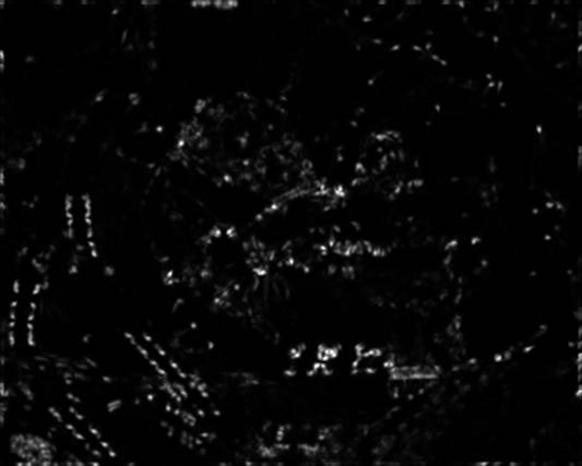
Figure 5. Harris Values of “Graf” img1.ppm (harris.tga)

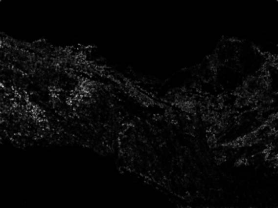
Figure 6. Harris Values of “Yosemite” Yosemite1.jpg (harris.tga)

Benchmark Results

Average AUC (Leuven)

Matching \ Descriptor	5x5 Window	MOPS
SSD	0.357021	0.702188
Ratio Test	0.557175	0.727467

Average AUC (Bikes)

Matching \ Descriptor	5x5 Window	MOPS
SSD	0.356457	0.645929
Ratio Test	0.516427	0.649424

Average AUC (Wall)

Matching \ Descriptor	5x5 Window	MOPS
SSD	0.397541	0.682856
Ratio Test	0.564342	0.661867

Strengths and Weaknesses

By design, the simplified MOPS descriptor with the Harris corner detection is relatively invariant to translation (using small patches), rotation (using oriented patches), and affine intensity changes (normalizing pixel values). However, the implementation was not designed to be invariant to changes in image scale. Some other weaknesses include: (1) Limited feature detection near image boundaries (due to the 20 pixel cut-off mentioned in the design section) and (2) No invariance to 3D transformations.

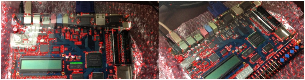
II. Additional Images

FPGA Features - Harris Detection, Simplified MOPS Descriptor, and Ratio Test Matching