Scott Cambo (sac355) & Karina Sobhani's(ks598) Project 2 - Feature Detection & Matching

a screenshot of my office
Design Features
Compute Harris Features
The major choice we made in this function was how to compute the angleRadians field for each features. We computed the angle by creating two gradients for the grayscale image: one in the x direction (Ix) and one in the y direction (Iy) using the sobel operators.
We then computed the angle by accessing the pixel pertaining to the feature in both the Ix and Iy gradient images. The angle was then computed as the following:
Angle = atan(Iy/Ix)
This works because the gradient shows the direction of most change which will give us the right angle of orientation. This may not have been the best way to calculate the angle.
Compute Harris Values
This function was written according to how the lecture slides presented computing the corner strength of each pixel. One choice we made was to check the trace of H. If the trace is 0, we set the corner strength to 0 since we don't want to divide by 0.
Compute Local Maxima
We set the threshold for detecting local maxima to be 0.1. This seems to give a reasonable number of features. A pixel is only set to 1 if its harris corner strength is both a local maximum and greater than the threshold.
ComputeMOPsDescriptors
The major choices we made involved transforming the image so that we could obtain the correct 8x8 window for each feature.
To transform a basic 8x8 image (output) at the origin to the location and size of the 41 by 41 window (gaussianImage), we took the following steps:
- Translate the 8x8 window so that the window is centered at the origin. This is done by translating the window by -8/2 in both the x and y direction.
- Scale the 8x8 window by 41/8. This makes the 8x8 window, a window of size 41x41.
- Rotate the image by angleRadians (the field computed in the feature). This orients the 8x8 window into the same orientation as the original 41x41 window.
- Translate the image by f.x in the x direction and f.y in the y direction (where f is the feature). This brings the output 8x8 window to the same location as the input 41x41 window.
We then used WarpGlobal by combining these transformations into one transformation: xform. This in effect gives us a nice 8x8 window at the origin for each feature. The reason we combined the transformations into one is because it is both faster and more accurate since the image will be sampled less.
Strengths and Weaknesses
One weakness is computing the angle of orientation for the feature. There is probably a better way to do it then via the gradient method that we used. As you can see in the gui, the matches are not as accurate as they could be.
Neither of us are too strong with C++, but we are getting better at the programming and the mathematical concepts as the course progresses. The math is both really interesting and fundamental to Computer Vision.
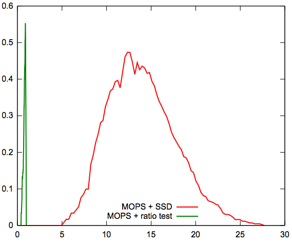
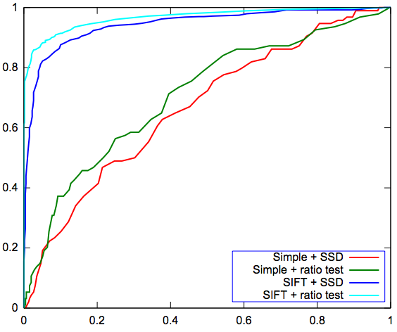
Metrics
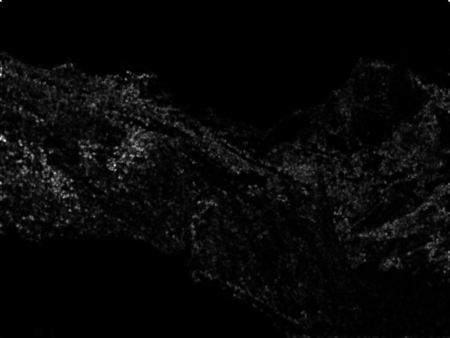
Graf
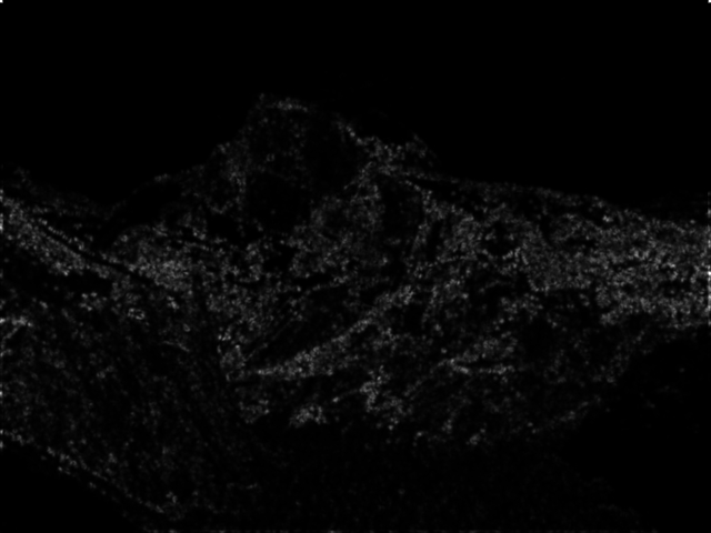

Yosemite


Benchmarks
Bikes
average error: 426.017459 pixels
average AUC: 0.604274
Leuven
average error: 310.278898 pixels
average AUC: 0.590297
Wall
average error: 277.009201 pixels
average AUC: 0.584067