Design Choices
We made major design choices in some of the methods that we were tasked with writing, while others only required
basic code to go over a window around each pixel and do some slightly different calculations.
The only part of ComputeHarrisFeatures that we changed was in the final section that fills in each feature. Here
we were tasked with inputting id, type, x ,y and angle. The ids were simply incrementing a variable, the type was
2 for harris features, x and y came from the pixel, and angle was the only value that required additonal
computation. To set the angle field, we developed a bin system wherein each feature was placed into a bin based on
which bin it's true angle fell inside. This was done so that later in MOPS descriptor computation we would only
have to warp the original image once for each bin and use it for each feature that fell into the bin. The original
angle of a feature was determined by calculating the gradients for all the pixels in a window around the pixel
designated as the feature's center. Each of these values from surrouding pixels was then weighted based on its
magnitude and a gaussian matrix designed to make the result invariant to rotation. Once the values from each pixel
in the window have been calculated, the bin represented most heavily in the window becomes the bin associated with
the feature, and the angle of the feature is set as the angle representing the middle of the bin. We chose to
submit with 50 bins, which only leaves 7.2 degrees to be covered in each bin, a relatively small amount. The trade
off here is between speed and correctness and we decided to chose a bin number that results in slightly slower
performance than the solution code, but also slightly better results.
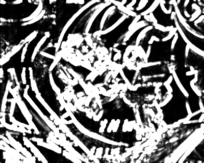
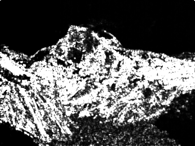
We were responsible for completing computeHarrisValues so that it correctly gave each pixel a value based on the
harris matrix we defined. We formed our harris matrix for each pixel by first computing the gradients with sobel
filters and combining the results with gaussian weighting. The members of the matrix were I_x * I_x * weight, I_x
* I_y * weight, and I_y * I_y * weight. Once these were computed using each pixel in a window around our current
pixel, the determinant and trace were found for the matrix, and the harrisvalue of the pixel was set as
determinant/trace. When a pixel in the window was considered to be out of bounds, we used the center pixel values
in its place.
In computeLocalMaxima, we used a variation on our basic "for every pixel got through a window around the pixel"
code. The difference here is what we did inside the center and how we handled out of bounds issues. In this case
since we are looking for maxima, we can ignore any pixels outside the area because we know they are not maxima,
thus we jsut continue to the next iteration of the loop if we find this. Otherwise if a pixel can survive going
through all its neighbors without finding a value greater than itself, it is marked as a local max in the output
image.
The code that went into ComputeSimpleDescriptors was also a variation on going through a window around every pixel.
The main difference here is that we duplicate the center pixel if we find ourselves out of bounds and when
inbounds we simply record the pixel information in the corresponding index of the data vector.
Arguably the most work and decisions went into completing ComputeMOPSDescriptors. To begin the computation, we
take the input image and turn it to gray scale before blurring it. We then use this image in the rest of our
computations. The general idea here is that we make use of the bins that all our features have been placed in,
back in compute harris features. This allows us to lump together features and reduce the total number of warps(
calls to warpGlobal()) that we have to make. Our outer loop executes once for each bin we have, and the warp that
occurs is consequently different, specifically in the rotation portion of the transformation matrix that is passed
in. The warp takes in the whole image and produces an image of larger size, so as to accomodate whatever rotation
has been passed in and to allow all the features with that rotation to gether data from this one warped image. To
this end, we have a loop going through each feature within the outer warping loop. Here we determine if the
feature matches the current orientation or not. If it does not, we continue, if it does then we execute code very
similar to the simple descriptor in which we record a window around the pixel. The difference is that this patch
is 8x8 and is downsampled from a larger 41 by 41 area taken out of our blurred and rotated warp result. This
provides rotational invariance and is what makes mops an improvement over the simple descriptor.
The final change that we made was in the ratioMatchFeatures method. This is very similar to the code in
ssdMatchfeatures with a few changed. The most important is that the score is determined by a ratio of the first
and second best matches instead of simply being decided by the best match. Therefore we had to modify the code to
keep track of the second best match while also keeping track of the best. The ratio distance is then the best
distance divided by the second best distance.


