Priority Queues and Heaps

For Dijkstra's shortest-path algorithm, we needed a priority queue: a queue whose elements are removed in priority order. A priority queue is an abstraction with several important uses. And it can be implemented efficiently, as we'll see.

We've already seen that priority queues are useful for implementing Dijkstra's algorithm and A^* search. Priority queues are also very useful for event-driven simulation, where the simulator needs to handle events in the order in which they occur, and handling one event can result in adding new events in the future, which need to be pushed onto the queue. Another use for priority queues is for the compression algorithm known as Huffman coding, the optimal way to compress individual symbols in a stream. Priority queues can also be used for sorting, since elements to be sorted can be pushed into the priority queue and then removed in sorted order.

Priority queue interface

A priority queue can be described via the following interface:

PriorityQueue.java

This interface suffices to implement Dijkstra's shortest path algorithm, for example.

Implementing increasePriority() requires that it be possible to find the element in the priority queue. This can be accomplished by using a hash table to look up element locations, or by augmenting the elements themselves with an extra instance variable that holds their location. We largely ignore that issue here.

Implementation 1: Binary Search Tree

One simple implementation of a priority queue is as a binary search tree, using element priorities as keys. New elements are added by using the ordinary BST add operation. The minimum element in the tree can be found by simply walking leftward in the tree as far as possible and then pruning or splicing out the element found there. The priority of an element can be adjusted by first finding the element; then the element is removed from the tree and readded with its new priority. Assuming that we can find elements in the tree in logarithmic time, and that the tree is balanced, all of these operations can be done in logarithmic time, asymptotically.

Implementation 2: Binary Heap

However, a balanced binary tree is overkill for implementing priority queues; it is conventional to instead use a simpler data structure, the binary heap. The term heap is a bit overloaded; binary heaps should not be confused with memory heaps. A memory heap is a low-level data structure used to keep track of the computer's memory so that the programming language implementation knows where to place objects in memory.

A binary heap, on the other hand, is a binary tree satisfying the heap order invariant:

(Order) For each non-root node n, the priority of n is no higher than the priority of n's parent. Equivalently, a heap stores its minimum element at the root, and the left and right subtrees are also both heaps.

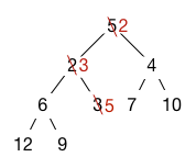
Here is an example of a binary heap in which only the priorities of the elements are shown:

Notice that the root of each subtree contains the highest-priority element.

It is possible to manipulate binary heaps as tree structures. However, additional speedup can be achieved if the binary heap satisfies a second invariant:

(Shape) If there is a node at depth h, then every possible node of depth h–1 exists along with every possible node to the left of depth h. Therefore, the leaves of the tree are only at depths h and h–1. This shape invariant may be easier to understand visually:

In fact, the example tree above also satisfies this shape invariant.

The reason the shape invariant helps is because it makes it possible to represent the binary heap as a resizable array. The elements of the array are “read out” into the heap structure row by row, so the heap structure above is represented by the following array of length 9, with array indices shown on the bottom.

How is it possible to represent a tree structure without pointers? The shape invariant guarantees that the children of a node at index i are found at indices 2i+1 (left) and 2i+2 (right). Conversely, the parent of a node at index i is found at index (i–1)/2, rounded down. So we can walk up and down through the tree by using simple arithmetic.

Binary heap operations

Add

Adding is done by adding the element at the end of the array to preserve the Shape invariant. This violates the Order invariant in general, though. To restore the Order invariant, we bubble up the element by swapping it with its parent until it reaches either the root or a parent node of higher priority. This requires at most lg n swaps, so the algorithm is O(lg n). For example, if we add an element with priority 2, it goes at the end of the array and then bubbles up to the position where 3 was:

ExtractMin

The minimum element is always at the root, but it needs to be replaced with something. The last element in the array needs to go somewhere anyway, so we put it at the root of the tree. However, this breaks the order invariant in general. We fix the order invariant by bubbling the element down. The element is compared against the two children nodes and if either is higher-priority, it is swapped with the higher priority child. The process repeats until either the element is higher-priority than its children or a leaf is reached. Bubbling down ensures that the heap order invariant is restored along the path from the root to the last heap element. Here is what happens with our example heap:

IncreasePriority

Increasing the priority of an element is easy. After increasing the priority, we simply bubble it up to restore Order.

HeapSort

The heapsort algorithm sorts an array by first heapifying it to make it satisfy Order. Then extractMin() is used repeatedly to read out the elements in increasing order.

Heapifying can be done by bubbling every element down, starting from the last non-leaf node in the tree (at index n/2 - 1) and working backward and up toward the root:

for (i = (n/2)-1; i >= 0; i--) {
    bubble_down(i);
}

The total time required to do this is linear. At most half the elements need to be bubbled down one step, at most a quarter of the elements need to be bubbled down two steps, and so on. So the total work is at most n/2 + 2·n/4 + 3·n/8 + 4·n/16 + ..., which is O(n).

Treaps

A treap is a binary search tree that is balanced with high probability. This is achieved by ensuring the tree has exactly the same structure that it would have had if the elements had been inserted in random order. Each node in a treap contains both a key and a randomly chosen priority. The treap satisfies the BST invariant with respect to all of its keys so elements can be found in the treap in logarithmic time. The treap satisfies the heap invariant with respect to all its priorities. This ensures that the tree structure is exactly what you'd get if the elements had been inserted in priority order.

For example, the following is a treap where the keys are the letters and the priorities are the numbers.

Elements are added to the treap in the usual way for binary search trees. However, this may break the Order invariant on priorities. To fix that invariant, the element is bubbled up through the treap using tree rotations that swap a node with its parent while preserving the BST invariant. If the node is x and it is the right child of a parent p, the tree rotation is performed by changing pointers so the data structure on the left turns into the data structure on the right.

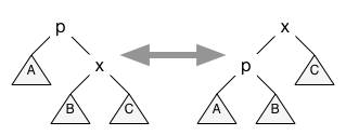
Notice that A, B, and C here represent entire subtrees that are not affected by the rotation except that their parent node may change. Conversely, if the node is p and it's the left child of a parent x, the tree rotation to swap p with x transforms the data structure on the right to the one on the left.

For example, adding a node D with priority 2 to the treap above results in the following rotations being done to restore the Order invariant:

Notice that this is exactly the tree structure we'd get if we had inserted all the nodes into a simple BST in the order specified by the priorities of the nodes.