Graphs and graph representations
Topics:
- vertices and edges
- directed vs undirected graphs
- labeled graphs
- adjacency and degree
- adjacency-matrix and adjacency-list representations
- paths and cycles
- topological sorting
- more graph problems: shortest paths, graph coloring
A graph is a highly useful mathematical abstraction. A graph consists of a set of vertices (also called nodes) and a set of edges (also called arcs) connecting those vertices. There are two main kinds of graphs: undirected graphs and directed graphs. In a directed graph (sometimes abbreviated as digraph), the edges are directed: that is, they have a direction, proceeding from a source vertex to a sink (or destination) vertex. The sink vertex is a successor of the source, and the the source is a predecessor of the sink. In undirected graphs, the edges are symmetrical.

Uses of graphs
Graphs are a highly useful abstraction in computer science because so many important problems can be expressed in terms of graphs. We have already seen a number of graph structures: for example, the objects in a running program form a directed graph in which the vertices are objects and references between objects are edges. To implement automatic garbage collection (which discards unused objects), the language implementation uses a algorithm for graph reachability.
Other examples of graphs, many of which we've seen, include:
- states of games and puzzles, which are vertices connected by edges that are the legal moves in the game,
- state machines, where the states are vertices and the transitions between states are edges,
- road maps, where the vertices are intersections or points along the road and edges are roads connecting those points,
- scheduling problems, where vertices represent events to be scheduled and edges might represent events that cannot be scheduled together, or, depending on the problem, edges that must be scheduled together,
- and in fact, any binary relation ρ can be viewed as a directed graph in which the relationship x ρ y corresponds to an edge from vertex x to vertex y.
What is the value of having a common mathematical abstraction like graphs? One payoff is that we can develop algorithms that work on graphs in general. Once we realize we can express a problem in terms of graphs, we can consult a very large toolbox of efficient graph algorithms, rather than trying to invent a new algorithm for the specific domain of interest.
On the other hand, some problems over graphs are known to be intractable to solve in a reasonable amount of time (or at least strongly suspected to be so). If we can show that solving the problem we are given is at least as hard as solving one of these
Vertices and edges
The vertices V of a graph are a set; the edges E can be viewed as set of ordered pairs (v1, v2) representing an edge with source vertex v1 and sink vertex v2.
If the graph is undirected, then for each edge (v1, v2), the edge set also includes (v1, v2). Alternatively, we can view the edges in an undirected graph as a set of sets of edges {v1, v2}.
Edges from a vertex to itself may or may not be permitted depending on the setting; also, multiple edges between the same vertices may be permitted in some cases.
Adjacency and degree
Two vertices v and w are adjacent, written v ~ w, if they are connected by an edge. The degree of a vertex is the total number of adjacent vertices. In a directed graph, we can distinguish between outgoing and incoming edges. The out-degree of a vertex is the number of outgoing edges and the in-degree is the number of incoming edgs.
Labels
The real value of graphs is obtained when we can use them to organize information. Both edges and vertices of graphs can have labels that carry meaning about an entity represented by a vertex or about the relationship between two entities represented by an edge. For example, we might encode information about three cities, Syracuse, Ithaca, and Binghamton as edge and vertex labels in the following undirected graph:

Here, the vertices are labeled with a pair containing the name of the city and its population. The edges are labeled with the distance between the cities.
A graph in which the edges are labeled with numbers is called a weighted graph. Of course, the labels do not have to represent weight; they might stand for distance betweenvertices, or the probability of transitioning from one state to another, or the similarity between two vertices, etc.
Graph representations
There is more than one way to represent a graph in a computer program. Which representation is best depend on what graphs are being represented and how they are going to be used. Let us consider the following weighted directed graph and how we might represent it:

Adjacency matrix
An adjacency matrix represents a graph as a two-dimensional array. Each
vertex is assigned a distinct index in [0, |V|). If
the graph is represented by the 2D array m, then the
edge (or lack thereof) from vertex i to vertex j
is recorded at m[i][j].
The graph structure can be represented by simplying storing a boolean value at each array index. For example, the edges in the directed graph above are represented by the true (T) values in this matrix:
| 0 | 1 | 2 | 3 | |
|---|---|---|---|---|
| 0 | F | T | T | F |
| 1 | F | F | F | T |
| 2 | F | T | F | T |
| 3 | F | F | F | F |
More compact bit-level representations for the booleans are also possible.
Typically there is some information associated with each edge; instead of a boolean, we store that information into the corresponding array entry:
| 0 | 1 | 2 | 3 | |
|---|---|---|---|---|
| 0 | — | 10 | 40 | — |
| 1 | — | — | — | –5 |
| 2 | — | 25 | 20 | — |
| 3 | — | — | — | — |
The space required by the adjacency matrix representation is O(V2), so adjacency matrices can waste a lot of space if the number of edges |E| is O(V). Such graphs are said to be sparse. For example, graphs in which in-degree or out-degree are bounded by a constant are sparse. Adjacency matrices are asymptotically space-efficient, however, when the graphs they represent are dense; that is, |E| is O(V2).
The adjacency matrix representation is time-efficient for some operations. Testing whether there is an edge between two vertices can clearly be done in constant time. However, finding all incoming edges to a given vertex, or finding all outgoing edges, takes time proportional to the number of vertices, even for sparse graphs.
Undirected graphs can be represented with an adjacency matrix too, though the matrix will be symmetrical around the matrix diagonal. This symmetry invariant makes possible some space optimizations.
Adjacency list representation
Since sparse graphs are common, the adjacency list representation is often preferred. This representation keeps track of the outgoing edges from each vertex, typically as a linked list. For example, the graph above might be represented with the following data structure:
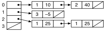
Adjacency lists are asymptotically space-efficient because they only use space proportional to the number of vertices and the number of edges. We say that they require O(V+E) space.
Finding the outgoing edges from a vertex is very efficient in the adjacency list representation too; it requires time proportional to the number of edges found. However, finding the incoming edges to a vertex is not efficient: it requires scanning the entire data structure, requiring O(V+E) time.
When it is necessary to be able to walk forward on outgoing edges and backward on incoming edges, a good approach is to maintain two adjacency lists, one representing the graph as above and one corresponding to the dual (or transposed) graph in which all edges are reversed. That it, if there is a an edge a→b in the original graph, there is an edge b→a in the transposed graph. Of course, an invariant must be maintained between the two adjacency list representations.
Testing whether there is an edge from vertex i to vertex j requires scanning all the outgoing edges, taking O(V) time in the worse case. If this operation needs to be fast, the linked list can be replaced with a hash table. For example, we might implement the graph using this Java representation, which preserves the asympotic space efficiency of adjacency lists while also supporting queries for particular edges:
HashMap<Vertex, HashMap<Vertex, Edge>>
Paths and cycles
Following a series of edges from a starting vertex creates a walk through the graph, a sequence of vertices (v0,...,vp) where there is an edge from vi-1 to vi for all i between 1 and p. The length of the walk is the number of edges followed (that is, p). If no vertex appears twice in the walk, except that possibly v0 = vn, the walk is called a path. If there are no repeating vertices, it is a simple path. If the first and last vertices are the same, the path is a cycle.
Some graphs have no cycles. For example, linked lists and trees are both examples of graphs in which there are no cycles. They are directed acyclic graphs, abbreviated as DAGs. In trees and linked lists, each vertex has at most one predecessor; in general, DAG vertices can have more than one predecessor.
Topological sorting
One use of directed graphs is to represent an ordering constraint on vertices. We use an edge from x to y to represent the idea that “x must happen before y”. A topological sort of the vertices is a total ordering of the vertices that is consistent with all edges. A graph can be topologically sorted only if it has no cycles; it must be a DAG.
Topological sorts are useful for deciding in what order to do things. For example, consider the following DAG expressing what we might call the “men's informal dressing problem”:

A valid plan for getting dressed is a topological sort of this graph, and in fact any topological sort is in principle a workable way to get dressed. For example, the ordering (pants, shirt, belt, socks, tie, jacket, shoes) is consistent with the ordering on all the graph edges. Less conventional strategies are also workable, such as (socks, pants, shoes, shirt, belt, tie, jacket).
Does every DAG have a topological sort? Yes. To see this, observe that every finite DAG must have a vertex with in-degree zero. To find such a vertex, we start from an arbitrary vertex in the graph and walk backward along edges until we reach a vertex with zero in-degree. We know that the walk must generate a simple path because there are no cycles in the graph. Therefore, the walk must terminate because we run out of vertices that haven't already been seen along the walk.
This gives us an (inefficient) way to topologically sort a DAG:
- Start with an empty ordering.
- Find a 0 in-degree node and put it at the end of the ordering built thus far (the first node we do this with will be the first node in the ordering).
- Remove the node found from the graph.
- Repeat from step 2 until the graph is empty.
Since finding the 0 in-degree node takes O(V) time, this algorithm takes O(V2) time. We can do better, as we'll see shortly.
Other graph problems
Many problems of interest can be expressed in terms of graphs. Here are a few examples of important graph problems, some of which can be solved efficiently and some of which are intractable!
Reachability
One vertex is reachable from another if there is a path from one to the other. Determining which vertices are reachable from a given vertex is useful and can be done efficiently, in linear time.
Shortest paths
Finding paths with the smallest number of edges is useful and can be solved efficiently. Shortest-path problems address a generalization: minimizing the total weight of all edges along a path, where the weight of an edge is thought of as a distance.
For example, if a road map is represented as a graph with vertices representing intersections and edges representing road segments, the shortest-path problem can be used to find short routes. There are several variants of the problem, depending on whether one is interested in the distance from a given root vertex or in the distances between all pairs of vertices. If negative-weight edges exist, these problems become harder and different algorithms (e.g., Bellman–Ford) are needed.
Hamiltonian cycles and the traveling salesman problem
The problem of finding the longest path between two nodes in a graph is, in general, intractable. It is related to some other important problems. A Hamiltonian path is one that visits every vertex in a graph. The ability to determine whether a graph contains a Hamiltonian path (or a Hamiltonian cycle) would be useful, but in general this is an intractable problem for which the best exact algorithms require exponential-time searching.
A weighted version of this problem is the traveling salesman problem (TSP), which tries to find the Hamiltonian cycle with the minimum total weight. The name comes from imagining a salesman who wants to visit every one of a set of cities while traveling the least possible total distance. This problem is at least as hard as finding Hamiltonian cycles. However, finding a solution that is within a constant factor (e.g., 1.5) of optimal can be done in polynomial time with some reasonable assumptions. In practice, there exist good heuristics that allow close-to-optimal solutions to TSP to be found even for large problem instances.
Graph coloring
Imagine that we want to schedule exams into k time slots such that no student has two exams at the same time. We can represent this problem using an undirected graph in which the exams are vertices. Exam V1 and exam V2 are connected by an edge if there is some student who needs to take both exams. We can schedule the exams into the k slots if there is a k-coloring of the graph: a way to assign one of k colors, representing the time slots, to each of the vertices such that no two adjacent vertices are assigned the same color.
The problem of determining whether there is a k-coloring turns out to be intractable. The chromatic number of a graph is the minimum number of colors that can be used to color it; this is of course intractable too. Though the worst case is intractable, in practice, graph colorings close to optimal can be found.