Priority Queues and Heaps

To implement Dijkstra's shortest-path algorithm, we need a priority queue: a queue in which each element has a priority and from which elements are removed in priority order; that is, the next element to be removed from the queue is always the element of highest priority currently in the queue. A priority queue is an abstraction with several important uses, and fortunately, it can be implemented efficiently.

We have already seen that priority queues are useful for implementing Dijkstra's algorithm and A^* search. In these applications, the priority is the best-known estimate of a shortest distance. Such a queue is called a min-queue because the smaller the distance, the higher the priority. There are also max-queues in which larger numbers correspond to higher priorities, but they can be implemented in the same way.

Another application in which priority queues are very useful is discrete event-driven simulation. Such a simulator needs to process events in the order in which they occur, updating the state of the simulation for each event. A min-queue is used to store unprocessed events, where the priority is a timestamp indicating the time of occurrence. Handling one event can generate new future events, which are added to the queue.

Another use for priority queues is for the data compression algorithm known as Huffman coding, an optimal way to compress individual symbols in a data stream. Priority queues can also be used for sorting, since elements to be sorted can be pushed into the priority queue and then simply removed in sorted order. In fact, with a good implementation of priority queues, this sorting algorithm is asymptotically optimal.

Priority queue interface

A priority queue can be described via the following interface:

PriorityQueue.java

The methods described in this interface suffice to implement Dijkstra's shortest path algorithm.

To implement increasePriority(), an implementation must have a fast way to find the element whose priority is to be updated. This can be accomplished by using a hash table to look up the position of elements in the underlying data structure, or by storing the position of the element in the queue into the element itself. Using the Concept design pattern, we would pass an object to the priority queue that provides operations for manipulating queue elements, providing an interface like the following:

ElemOps.java

Implementation 1: list

It is straightforward to implement priority queues with ordered or unordered lists. Ordered lists allow constant-time extractMin and linear time add, whereas unordered lists allow constant-time add and linear time extractMin. We can do better!

Implementation 2: Binary Search Tree

If you already have an implementation of balanced search trees, it is easy to implement priority queues on top. The idea is to use elements as keys, ordered first by their priorities and secondarily by the some intrinsic element ordering. New elements are added by using the ordinary BST add operation. The minimum element in the tree can be found by simply walking leftward in the tree as far as possible and then pruning or splicing out the element found there. The priority of an element can be adjusted by first finding the element; then the element is removed from the tree and readded with its new priority.

This implementation has reasonable asymptotic performance: all of the operations can be done in logarithmic time, asymptotically. However, a balanced search tree is unnecessarily complex for the priority queue job, and consequently a bit slow.

Implementation 3: Binary Heap

A simple concrete data structure called a binary heap allows all operations to be done in \(O(\log n)\) time with good constant factors.

In computer science, the term heap is unfortunately a bit overloaded. Binary heaps should not be confused with memory heaps. A memory heap is a low-level data structure used to keep track of the computer's memory so that the programming language implementation knows where to place objects in memory. This is not how we are using the term here.

A binary heap is a binary tree satisfying the heap invariant:

(Heap Invariant) Every node n in the tree has the highest priority among all nodes in the subtree rooted at n. Equivalently, the priority of any node is at least as high as the priority of any of its children. Equivalently still, a heap stores its highest priority element at the root, and the left and right subtrees are also both heaps.

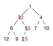
Here is an example of a binary heap in which smaller values have higher priority. Note that the root of each subtree contains the highest-priority element in that subtree.

It is possible to manipulate binary heaps as tree structures. However, additional speedup can be achieved if the binary heap satisfies a second invariant:

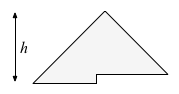
(Shape Invariant) For every h, if there exists a node n at depth h, then all 2^h-1 possible node of depth h–1 exist in the tree, along with every possible node to the left of n of depth h. It follows that if h is the maximum depth of a node in the tree, the leaves of the tree occur only at depths h and h–1.

In fact, the example tree above also satisfies this shape invariant.

The shape invariant makes it possible to represent the binary heap as a resizable array. The elements of the tree are placed in the array row by row from top to bottom, reading each row from left to right and placing the nodes in the array from left to right. The heap structure illustrated above would be represented by the following array of length 9, with array indices shown on the bottom.

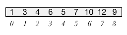
The nice thing about this representation is that it is possible to represent the tree structure without pointers. The shape invariant guarantees that the children of the node at index \(i\) are found at indices \(2i+1\) (left) and \(2i+2\) (right). Conversely, the parent of a node at index i is found at \(\lfloor (i–1)/2 \rfloor \). So we can walk up and down through the tree using simple arithmetic. There is no need to store or follow pointers!

Binary heap operations

Add

Adding a new node to the heap is done by adding the element at the end of the array to preserve the shape invariant. However, the heap invariant may not hold, because its priority may be greater than its parent's priority. To restore the heap invariant, we bubble up the element by swapping it with its parent until either it reaches the root or its parent node has higher priority. This requires at most \(\lg n\) swaps, because the tree is perfectly balanced. So adds take at most \(O(\log n)\) time.

In the example above, if we add an element with priority 2, it is first placed at the end of the array, then bubbles up past the 5 and the 3, finally ending up where 3 was:

ExtractMin

The minimum element is always at the root (location 0 in the array). We can extract it, but we need to replace it with something. The last element in the array is a good candidate. We move it to the root of the tree. This reestablishes the shape invariant, but the heap invariant may now be broken. We fix the heap invariant by bubbling the element down (sometimes also called sifting down). The element is compared against its two children. If either child is higher priority, it is swapped with the higher priority child. The process repeats until either the element is higher priority than its children or it becomes a leaf.

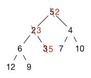
Here is what happens with our example heap. We delete the 1 at the root and replace it with 5, which was the last element in the array. Then we bubble the 5 down. We compare it with 2 and 4. It is lower priority than both, so we swap it with the higher priority child, which is 2. (We must swap it with the higher priority child to maintain the heap invariant, because that child will become the parent of the other child.) We then compare with the new children, 6 and 3, and swap with 3, at which point 5 becomes a leaf. The heap invariant is now reestablished.

Again, at most \(\lg n\) swaps are needed.

IncreasePriority

We may wish to change the priority of an element in the queue. Assigning a new priority to an element maintains the shape invariant, but may break the heap invariant. To reestablish the heap invariant, we may need to bubble the element up if we increase the priority (which for a min-queue means decreasing the value) or down if we decrease the priority.

Heapsort

The heapsort algorithm sorts an array by first heapifying it to make it satisfy the heap invariant. Then extractMin() is used repeatedly to read out the elements in increasing order. This can be used to sort an array in \(O(n \log n)\) time. That repeatedly calling extractMin() takes \(O(n \log n)\) time is obvious, but what about heapifying?

Heapifying can be done by bubbling every element down, starting from the last element in the array representation and working backward:

for (i = (n/2)-1; i >= 0; i--) {
  bubbleDown(i);
}

This loop works correctly because it has the following loop invariant: when the loop is considering node \(i\), the two subtrees of node \(i\) already satisfy the heap invariant: they occur in the part of the array that has already been scanned. Therefore, bubbling down node \(i\) is all that is needed to make the entire subtree rooted at \(i\) also satisfy the invariant.

The total time required to heapify is, perhaps surprisingly, linear. No work is done on the half of the elements in indices \(\lfloor n/2\rfloor\dots n-1\) because these are all leaves. Considering the rest of the elements, as suggested by the figure at the right, at most a quarter need to be bubbled down one step, at most an eighth need to be bubbled down two steps, and so on. So the total work is at most:

\begin{equation} T = n/4 + 2n/8 + 3n/16 + 4n/32 + \dots + kn/2^{k+1} + \dots \end{equation}

This series is easy to solve by taking the difference of two series in the usual way: \(T = 2T - T = n/2 + n/4 + n/8 + \dots = O(n) \).

Hence, we can see that heapifying is actually the fast part of heapsort!

Improvements

There are many variations on this basic data structure, some of which can yield significant performance improvements under the right circumstances.

When using priority queues to implement Dijkstra's shortest-path algorithm on dense graphs, the performance limiting operation is often increasePriority(), which as we have seen takes logarithmic time. Fibonacci heaps and relaxed heaps are heap data structures that can do increasePriority() in only constant (amortized) time, yielding a speedup. Since these data structures do not enforce the Shape invariant, they require pointers to implement. Hence, although their asymptotic performance is the same or better than a simple binary heap on all operations, they incur a higher constant factor slowdown that is typically not worth paying.

In many search applications, the binary heap will tend to contain a lot of elements with the same priority—especially, many elements with the same priority as the root. A simple optimization is to store all elements with the highest priority separately in a resizable array, significantly reducing the amount of bubbling down that is done by extractMin().

We can also exploit the linear-time performance of heapifying to make it cheaper to add new elements to a binary heap. Rather than immediately bubbling new elements up, we simply append them to a small unordered region of size \(O(\lg n)\) elements at the end of the array. For extractMin(), the smallest element could be in the unordered region, so it must scan these elements too—but this small scan takes logarithmic time and hence does not harm asymptotic performance. If the size of the unordered region becomes larger than \(O(\lg n)\) elements, we restore the heap invariant for the whole array by heapifying the unordered region into the rest of the array. If we heapify in a way that only touches the ancestors of the unordered regions, it takes \(O(\lg n)\) time and hence \(O(1)\) amortized time per element added.

Treaps

A treap is a binary search tree that is balanced with high probability. This is achieved by ensuring the tree has exactly the same structure that it would have had if the elements had been inserted in random order. Each node in a treap contains both a key and a randomly chosen priority. The treap satisfies the BST invariant with respect to all of its keys so elements can be found in the treap in (expected) logarithmic time. The treap satisfies the heap invariant with respect to all its priorities. This ensures that the tree structure is exactly what you would get if the elements had been inserted in priority order.

For example, the following is a treap where the keys are the letters and the priorities are the numbers.

Elements are added to the treap in the usual way for binary search trees. However, this may break the heap invariant on priorities. To fix the heap invariant, the element is bubbled up through the treap using tree rotations that swap a node with its parent while preserving the BST invariant. If the node is x and it is the right child of a parent p, the tree rotation is performed by changing pointers so the data structure on the left turns into the data structure on the right.

Note that A, B, and C here represent entire subtrees that are not affected by the rotation except that their parent nodes may change. Note also that the rotation operation is reversible, so that if p has higher priority than x, we can perform the rotation above from right to left.

Because they only affect three nodes of the tree, tree rotations are efficient:

Left rotation                          Right rotation
p.right = x.left;                      x.left = p.right;
x.left = p;                            p.right = x;
newChild = x;                          newChild = p;

For example, adding a node D with priority 2 to the treap above results in the following rotations being done to restore the heap invariant:

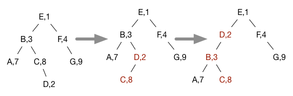
This is exactly the tree structure we would have gotten if we had inserted all the nodes into a simple BST in the order specified by their priorities.