
Figure 1: Invariant for the outer loop of insertion sort
Sorting a collection of values is a fundamental operation with many uses.
Let's look at the most common algorithms.
You might ask why we need to talk about sorting algorithms at all, given that
sorting algorithms are built into Java (see Arrays.sort) and many
other languages these days. One reasong is that it is useful to
understand the tradeoffs between different sorting algorithms.
Another is that at some point you will probably have to use
an environment in which sorting is not so available. Finally,
sorting is a great opportunity to talk about algorithms, loop invariants and
performance analysis.
Insertion sort is a simple algorithm that is the fastest way to sort small arrays. Intuitively, insertion sort scans through the array from left to right, making sure that the part of the array that has been scanned is always in sorted order. The code can be written as a loop with a loop invariant depicted as follows:
Figure 1: Invariant for the outer loop of insertion sort
The loop invariant is maintained by shifting each newly encountered element (at index i) leftward into the place it belongs in the sorted part of the array. This insertion causes the sorted part of the array to grow by one element. Eventually all elements have been inserted into the sorted part and there is nothing left to sort.
InsertionSort.java
The loop invariant for the outer loop is as depicted above. The invariant is satisfied when i=1 and each loop iteration ensures that the value that index i initially pointed to (k) is inserted into the right place.

Figure 2: Invariant for the inner loops
The invariant for the inner loop is also illustrated in the figure. The index j points to an array location such that everything to the left of j (region A) is less than everything to the right (region B). Further, everything in region B is greater than the value to be inserted, k. When the loop terminates, the top element in A is less than or equal to the k, so k can be placed in the element marked “?”. Figuring out loop invariants helps us write code like this that is efficient and correct.
The running time of insertion sort is best when the array is already sorted. In this case the inner loop stops immediately on each outer iteration, so the total work done per outer iteration is constant. Therefore the total work done by the algorithm is linear in the array size, which we write as O(n).
The worst case for the algorithm is when the array is sorted in the reverse order. In that case the loop on j goes all the way down to 0 on each outer iteration. The first iteration does two copies, the second three copies, and so on, so the total work is Σ {2,...,n} = n(n+1)/2 − 1. This function is O(n2), since O(n2+n) = O(n2).
Recall that in general, we can drop lower-order terms from polynomials when determining asymptotic complexity. For example, in this case (n2+n)/n2 limits to a constant (1) as n becomes large. Therefore the two functions in the ratio have the same asymptotic complexity.
Insertion sort has one other nice property: implemented properly, it is a stable sort, meaning that if given an array containing elements that are equal to each other, it keeps those elements in the same relative order as in the original array.
Selection sort is another sorting algorithm, used more commonly by humans than by computers. Intuitively, it tries to find the right element to put in each location of the final array. Once an array location is set to contain the right element, it is never changed.
for (int i = 0; i < n; i++) {
    // find smallest element in subarray a[i..n−1]
    // swap it with a[i]
}
Because each loop iteration must in turn iterate over the rest of the array to find the smallest element, the best-case performance of this algorithm is the same as the worst-case performance: O(n2).
More efficient sorting algorithms use recursion to implement a divide-and-conquer
strategy. They break the array into smaller subarrays and recursively
sort them. Merge sort is one such algorithm. Given an array to sort,
it finds the middle of the array and then recursively sorts the
left half and the right half of the array. Then it merges the
resulting arrays. A temporary array tmp is provided to give space
for merging work:
/** Sort a[l..r-1]. Modifies tmp.
    Requires: l < r, and tmp is an array at least as long as a.
 */
void sort(int[] a, int l, int r, int tmp[]) {
    if (l == r-1) return; // already sorted
    int m = (l+r)/2;
    sort(a, l, m, tmp);
    sort(a, m, r, tmp);
    merge(a, l, m, r, tmp)
}
The real work is done in merge, which takes time linear in the total
number of elements to be merged: O(r−l). It works by
scanning both subarrays to be merged from left to right, picking the smaller element
from each array as the following diagram suggests:

Array during merge
Here is the code. We use the notation a[l..r) to mean a[l..r-1].
/** Place a[l..r) into sorted order.
  * Requires: l < m < r, and a[l..m) and a[m..r) are both in sorted order.
  * Performance: O(r-l)
  */
void merge(int[] a, int l, int m, int r, int[] tmp) {
    int i = l, j = m, k = l;
    while (i < m && j < r)
        tmp[k++] = (a[i] < a[j]) ? a[i++] : a[j++];
    System.arraycopy(a, i, tmp, k, m-i);
    System.arraycopy(tmp, l, a, l, j-l);
}
At the end of the while loop, either i = m or
j=r, but not both, because only one of i
and j is incremented on each loop iteration. Therefore,
array a still contains some elements that have not been
copied to tmp, either in a[i..m) (if j = r)
or in a[j..r) (if i = m). if
j = r, the first arraycopy call
transfers the elements a[i..m) to tmp and the second
arraycopy copies all the elements from tmp back to a (since
j-l = r-l). If i=m, however,
elements in a[j..r), are already in the right place in
a, so there is no need to copy them to tmp and back again.
The first arraycopy does nothing, and the second
arraycopy copies just the elements tmp[l..j) into
a[l..j), leaving a[j..r) alone.
The running time of this algorithm is always O(n lg n), which is big improvement on O(n2). For example, if sorting a million elements, the speedup, ignoring constant factors, is 1,000,000/lg 1,000,000 ≈ 50,000. The speedup probably won't be quite that great when comparing to insertion sort because of constant factors.
To see why it is n lg n, think about the whole sequence of recursive calls shown in Figure 2. Each layer of recursive calls takes total merge time proportional to n, and there are lg n recursive calls. The total time spent in the algorithm is therefore O(n·lg n).
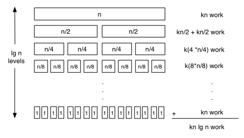
Figure 2: Merge sort performance analysis
Merge sort, like insertion sort, is a stable sort. This is a major reason when merge sort is commonly used. Another is that its run time is predictable.
Merge sort is not as fast as the quicksort algorithm that we will see
next because it does extra copying into the temporary array.
We can avoid some of the copying by exchanging the roles of a and tmp on
alternate recursive calls. This speeds up the algorithm at the cost of more complex code.
It is actually possible to do an in-place merge in linear time, but in-place merging
is tricky and is slower in practice than using a separate array.
Another trick that is used to speed up merge sort is to use insertion sort when the subarrays get small enough. For very small arrays insertion sort is faster, because k1n2 is smaller than k2n lg n when n and k1 are small enough!
Quicksort is another divide-and-conquer sorting algorithm. It avoids the work of merging by partitioning the array elements before recursively sorting. The algorithm chooses a pivot value p and then separates all the elements in the array so that the right half contains elements at least as large as p and the left half contains elements no larger than p.

Final partitioned state of the array
Thus, quicksort does some of the work of sorting before recursing. The two resulting subarrays can then be sorted recursively and the algorithm is done.
/** Sort a[l..r-1] */
void qsort(int[] a, int l, int r) {
    if (l == r-1) return; // base case: already sorted

    // partition elements around some pivot value p, obtaining partition index k
    int k = partition(a, l, r);

    qsort(a, l, k);
    qsort(a, k, r);
}
One thing we notice is that the choice of pivot matters. If the pivot
value is the largest or smallest element in the array, the subarrays
have lengths 1 and n−1. If this happens on every recursion—which
it easily can if the array is sorted to begin with—quicksort will
take O(n2) time. One solution is to choose the pivot randomly from
among the elements of the array, and swap it with a[l]. With this choice, quicksort has
expected run time O(n lg n), using reasoning similar to that for
merge sort. A different, commonly used heuristic is to choose the median of
the first, the last, and the middle element of the array. This
cheaper heuristic makes quicksort perform well on arrays that are mostly
sorted, while usually avoiding the O(n2) case in practice.
Now, how to partition elements efficiently? We want the array to end up looking like the diagram above. The idea is to start two pointers i and j from opposite ends of the array. They sweep in toward the middle swapping elements as necessary to achieve the final partitioned state shown above.
We start with the array containing the pivot value in its first element and the rest of the array in an unknown state:

Initial state of the array
The initial loop advances j so that it points to an element on the
wrong side of the array, with l ≤ i ≤ j < r:

State of the array at the start of the main loop
The loop must have an invariant that starts out describing this state but that
ends up describing the desired final state.
As the following diagram suggests, the invariant
says that all elements strictly to the left of i are at
most p, and all elements strictly to the right of
j are at least p. Further, the element at
i itself is at least p (and therefore belongs on the
right-hand side of the array) and the element at j
is at most p (and belongs on the left-hand side).
Finally, the inequalities l ≤ i ≤ j+1 ≤ r hold,
so both i and j are in bounds and can go past each other by at most a single index.
Therefore, if i and j do past each other,
the values they index will be on the correct side of the array and the
array can be partitioned between them.

Invariant during partitioning
Despite (or because of!) the complexity of the invariant, the partitioning code can then look very simple and be very efficient:
/** Partition array {@code a} into {@code a[l..k)} and {@code a[k..r)}, where {@code l<k<r}, and all elements
 * in {@code a[l..k)} are less than or equal to all elements in {@code a[k..r)}.
 * Requires: {@code 0≤l}, {@code r≤a.length}, and {@code r-l≥2}.
 */
int partition(int[] a, int l, int r) {
    int p = a[l]; // better: swap a[l] with random element first
    int i = l, j = r;
    do j--; while (a[j] > p);
    while (i < j) {
        swap a[i] ⇔ a[j]
        do i++; while (a[i] < p);
        do j--; while (a[j] > p);
    }
    return j+1;
}
The inner loops are written as do...while loops because we want to
do the body of each loop once even if the loop guard is initially false.
Interestingly, these inner loops do not need to do any bounds checking on
i and j. The reason bounds checks are not needed
is after swapping a[i] and a[j], there must be at
least one value “ahead” of both i and j that will
stop their inner loops.
An example of partitioning will probably help understand what is going
on. We start out with the following array, with p=5:
5 2 6 7 1 9 3 8
i               j
Before the main loop starts, we move j down to a value that can be swapped
with the pivot at index i:
5 2 6 7 1 9 3 8
i           j
In the first iteration, we swap and then move i and j inward to the next swappable values:
3 2 6 7 1 9 5 8
    i   j
In the second iteration, we swap and then move i and j inward again:
3 2 1 7 6 9 5 8
    j i
Since i > j,
the loop halts and the result is j+1 = 3. The two subarrays
to be recursively sorted are (3,2,1) and (7,6,9,5,8).
The loop can either stop with i = j+1 or with
i = j in the case where a[i] =
a[j] = p. Since j must be decremented at least twice,
either by the initial loop or by the first iteration of the main loop,
the value j+1 will always be a valid array index.
Quicksort is an excellent sorting algorithm for many applications. However, one downside is that it is not a stable sort. As with merge sort, it makes sense to switch to insertion sort for sufficiently small subarrays.
Finding the maximum and minimum elements in an array is a straightforward O(n) algorithm. But what if we want to find the median element? Or the 10th largest element? The problem of finding the nth largest element in an array is called the order statistics problem. Clearly, we can solve this problem by sorting the array and then indexing to the appropriate position, but that does a lot of sorting work that is not necessary.
Fortunately, the quicksort algorithm can be tweaked a little to solve the order statistics problem efficiently.
/** Returns: the nth largest element in the subarray {@code a[l..r)}
 *  Requires: {@code 0 ≤ n < r-l} and {@code l ≤ r < a.length} */
int qselect(int[] a, int l, int r, int n) {
    if (l+1 == r) return a[l];
    int k = partition(a, l, r);
    if (n < k)
        return qselect(a, l, k, n);
    else
        return qselect(a, k, r, n);
}
If partitioning perfectly splits the array in half each time, the total work is proportional to the finite geometric series n + n/2 + n/4 + ... + 1 = 2n− 1, which is O(n). Of course, the split won't usually be perfect, but the average split will still result in a series that is O(n). Therefore, expected time is O(n); worst-case time is, as with quicksort, O(n2).
Unlike quicksort, this method is tail-recursive, so it can be converted to a loop in the usual way, to obtain efficient
/** Returns: the nth largest element in the subarray {@code a[l..r)}
 *  Requires: {@code 0 ≤ n < r-l} and {@code l ≤ r < a.length} */
int qselect(int[] a, int l, int r, int n) {
    while (l+1 < r) {
        int k = partition(a, l, r);
        if (n < k) r = k;
        else l = k;
    }
    return a[l];
}