Image sharpening
When taking photographs, it’s not uncommon for the image to look blurry, especially when looked at up close. Shaky cameras, missed focus, and imperfect lenses all contribute. Fortunately, there are algorithms to reduce this blurriness by sharpening the image. In this project, you will implement one of these algorithms and apply it to a user-specified region of an image file.
We use some of the ideas from the filtering and edge detection examples in §12.4 of Insight. We discussed in lecture that median filtering was superior to mean filtering for noise reduction—the mean filter just makes the image blurry without removing much noise at all. In order to perform image sharpening, however, we actually need to start by making a blurry, e.g., mean-filtered, image. Then by subtracting the blurry image from the original, we get what can be called the “detail” of the image:

Notice that the “detail” is similar to what we call “edges” in §12.4. Now if we add some amount of the detail back to the original image, the result looks “sharpened.”

Image smoothing
Implement the function smoothImage() as specified below:
function smoothed = smoothImage(img, r)
% Smooth an image by averaging neighborhoods.
% `img` is a 3D uint8 array representing the color image to be smoothed.
% Smoothing is done using a mean filter with a neighborhood radius of `r` (a
% positive integer). Assume r < n/2 where n is the smaller of the number of
% rows and the number of columns of `img`.  The result, `smoothed`, should be
% a 3D uint8 array of the same size as `img`.
In lecture, we saw how to process data in the “neighborhood” of a pixel. We noted that, near the boundaries of the image, a full neighborhood was not available. Our solution then was to shrink the size of the neighborhood so that it fit within the image.
This time you’ll take a different approach. Before smoothing, you will pad the image array with extra rows and columns around the edges as necessary such that the neighborhood of every original pixel can have the same size. Here’s an example for a 2D case:
The original set of data contains 10×14 pixels, shown in white. If a radius-2 neighborhood is to be used, than a “padding” 2 pixels thick needs to be used, shown in yellow. An example radius-2 neighborhood is drawn above for pixel (10,4)—the original edge pixel (10,4)—and it has the same size, 5×5, as the neighborhood of any interior pixel.
What values should you use in the padding? The same values in the edge pixels of the original array. First concatenate side by side the leftmost column of the original array, the original array, and the rightmost column of the original array. This gives you a matrix 2 columns wider than the original (one extra column on each side). Next, concatenate to get a matrix 2 rows taller. Now you have a padding 1 pixel thick around the original matrix. Repeat as necessary to get the padding thickness that is needed. For a 3D array, pad every layer in the same way.
Include the padding procedure as a subfunction in smoothImage.m. You get to decide on the details of the function header; be sure to document its specification.
To speed up program the smoothing operation, you can use vectorized code and the built-in function sum() as appropriate. Note that sum() works in type double and returns values of type double; consider the following statements for example:
a= [100 200];  % array of type double
b= uint8(a);   % array of type uint8
c= sum(b);     % c stores the value 300, type double
d= uint8(c);   % d stores the value 255, type uint8
To sum the values in a 1D array, call the function sum as shown above. To sum the values in a 2D or 3D array A, call the function like this: sum(sum(A)). sum(A) returns a row vector such that the kth component is the sum of the kth column in matrix A. Summing this row vector then gives the sum of the matrix A. If A is 3-dimensional, this double-sum will return a 1×1×3 array containing the sum of each layer separately.
Be careful that you compute the smoothing only for the original pixels—the smoothed array that is returned must have the same size as the original array.
Image sharpening
Next, implement the following function:
function sharp = sharpenImage(img, smooth, w)
% Sharpen the image represented by the 3D uint8 array `img`.
% Requires a smoothed version of that image, `smooth`, a 3D uint8 array of the
% same size.  Sharpening is done by weighting (scaling) the difference between
% `img` and `smooth` by the factor w and adding this weighted difference to
% `img`, storing the result in `sharp`, also a 3D uint8 array of the same size.
This function is essentially the code that corresponds to the sequence of diagrams shown above. The calculations need to be done in type double in order to preserve the negative values from the subtraction. Recall that you can use the type name as a function to change the type of a variable, e.g., double(P) returns the values in P as an array of type double. The difference (original data minus the smoothed data) is then multiplied by the weight w and added to the original data. These operations may result in values that are outside the range [0,255]. When you set the type of the final array to uint8, any value that is less than 0 is truncated to 0 and any value that is greater than 255 is truncated to 255.
Sharpening a selected region
Finally, implement this function to create an interactive selective-sharpening tool:
function pic = sharpenRegion(imgfile, r, w)
% Sharpen (a part of) the image in the file named `imgfile` and return the
% uint8 array representing the (partially) sharpened image as `pic`.
% Image sharpening is based on a filter with neighborhood radius `r` and a
% weight `w` used to scale the image "detail."  `pic` has the size of the image
% named by file `imgfile`.
% Display the original image for the user to select an area for sharpening and
% display the final image in a separate figure.
This function reads the image data from the file named by imgfile, displays the image, allows the user to select a rectangular area, calls functions smoothImage() and sharpenImage() to sharpen the selected area of the image, and displays the entire image which is (partially) sharpened.
Using the title() function, prompt the user to click two points to select an area for sharpening. The two clicks are the opposing corners of a rectangle with sides parallel to the x- and y-axes. (The first click may be any corner, not necessarily top-left.) Use function ginput() to accept the mouse clicks, which are returned as x-y values. You need to round these values in order to use the x-value as a column number and the y-value as a row number. Furthermore, if a user clicks on the gray area outside the image, you should use the nearest valid column and row numbers for the image (these adjustments may be a good candidate for a subfunction…). See the section “Row and column indices vs. xand y-coordinates” below for more information on using ginput() on images. Sharpen only the part of the image selected by the user but display the entire final image, partially sharpened as specified by the user, in a separate figure window. Label both figures using the title area. The command figure opens a new figure window.
Row and column indices vs. x and y coordinates
The statement [xvec, yvec]= ginput(n) accepts n user mouseclicks on the current figure window and returns the x- and y- coordinates of the clicks in length n vectors xvec and yvec such that (xvec(1),yvec(1)) are the coordinates of the first click, (xvec(2),yvec(2)) are the coordinates of the second click, etc. In a typical figure window with Cartesian axes, x values increase to the right while y values increase going up. However, image data is stored in an array such that the top row of pixels of the image corresponds to row number 1, the row below that is row number 2, and so forth. Notice that the row number increases going down an image. The imshow() function flips the direction of the y-axis to match the image convention.
When we use built-in function ginput() to obtain the locations of the mouseclicks in a figure window displaying image array data, the “x-coordinate” returned corresponds to the column number of the pixel clicked while the “y-coordinate” returned corresponds to the row number of the pixel clicked. If you compare the returned “y-coordinates” of two clicks made one below the other on an image, you will see that the lower clicked location has the larger row number. Meanwhile, the column numbers increase to the right, like the x-axis. Note the difference in order: when we use coordinates we (usually) say x first and then y, but when you access an element in an array you specify row (corresponding to y) first and then column (corresponding to x). Be careful not to mix them up in your code—use meaningful names for your variables so that it’s crystal clear whether a variable refers to a coordinate or an index!
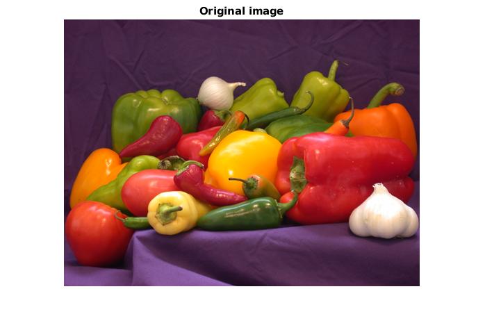
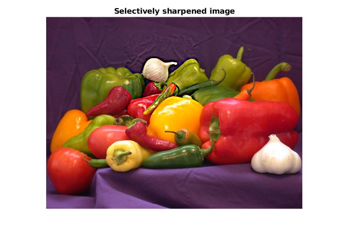
Image filtering is a compute-intensive operation, so throughout this project you should try to be efficient generally. As you develop your code, use a small image (or select a small area of an image) and a small filter radius (e.g., 1 or 2) to speed up testing. Be sure to try a bigger image and a bigger radius value (e.g., 5) after successful initial testing. Given our use of a mean-filter for smoothing, a good weight to use is 2, although it’s ok to try other values. Below are some resulting figures when calling this function on Matlab’s peppers.png image:


Notice the additional detail on the center onion’s skin, while the one in the bottom-right looks unchanged.