Working with Vectors
When calculating physical systems, we would like mathematical language and terms to describe properties of physical objects. In particular, it is important to be able to describe things like the position, direction, and/or speed of objects when doing calculations.
To describe these properties, we frequently talk about points, vectors,
and scalars. These are mathematical objects with operations that allow us to
put structure on physical systems. In this short tutorial, we will look at each
of these concepts, highlighting the standard operations for each. We also
show how the module introcs supports each of these concepts.
Points
A physical object exists at a point in space. We describe this point as the position of the object. For simplicity, we will assume that any point is in two dimensions, so each point has exactly an x and y coordinate. We represent a point on an xy-plane simply by drawing a dot at the x and y coordinates of the point:
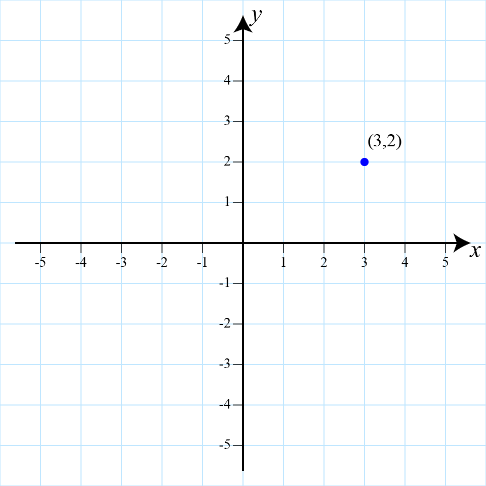
Point at (3,2)
Points in introcs are represented by the Point2
class. Objects of this class have attributes for the
Vectors
At the core of any physical system is movement. A vector describes movement of an object through two attributes: direction and magnitude. A vector can exist in any dimension, but again we focus just two dimensions. This means that our vectors are drawn in the xy-plane. Such vectors are drawn as an arrow starting at one position (often the origin), pointing to another position. The direction is the angle of the arrow counterclockwise from the x-axis, while the magnitude is the length of this arrow.
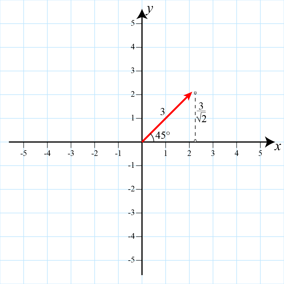
Vector with angle π/4 (45°) and magnitude 3
Vector Representation
This definition of a vector makes sense visually, but we need some way represent a
vector mathematically. There are two different ways to do this. One is to assume the
vector starts at the origin. We think represent the vector as
But as we said, vectors represent magnitude and direction. So we could also represent
a vector as a pair
We can go back and forth between the two representations with a little trigonometry.
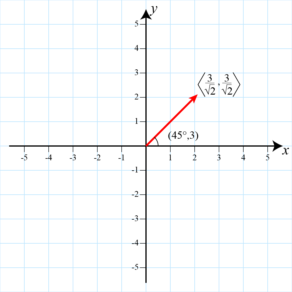
Representations of vector (
With that said, we often do not have to do these calculations ourselves, because Python
can do them for us. Vectors in introcs are represented by the Vector2
class. This class uses the “angle-bracket notation”. All objects have an
Vector Operations
A vector is applied to a point by simply adding the vector “arrow” to the current object position. Visually, this is simply a matter of moving the point along the path indicated by the arrow.
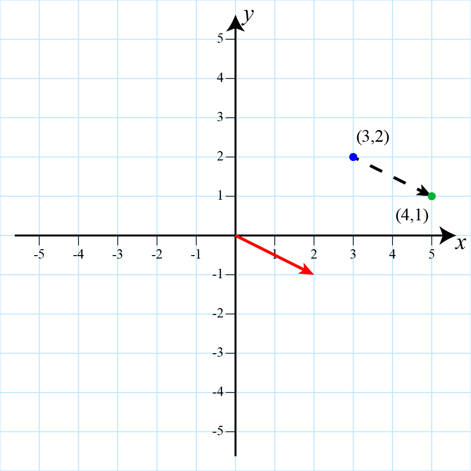
Applying a vector (in red) to the initial point (blue).
The resulting point is highlighted in green.
Vectors can be reversed (or more generally change direction) by simply producing
a new vector with the same magnitude but opposite direction
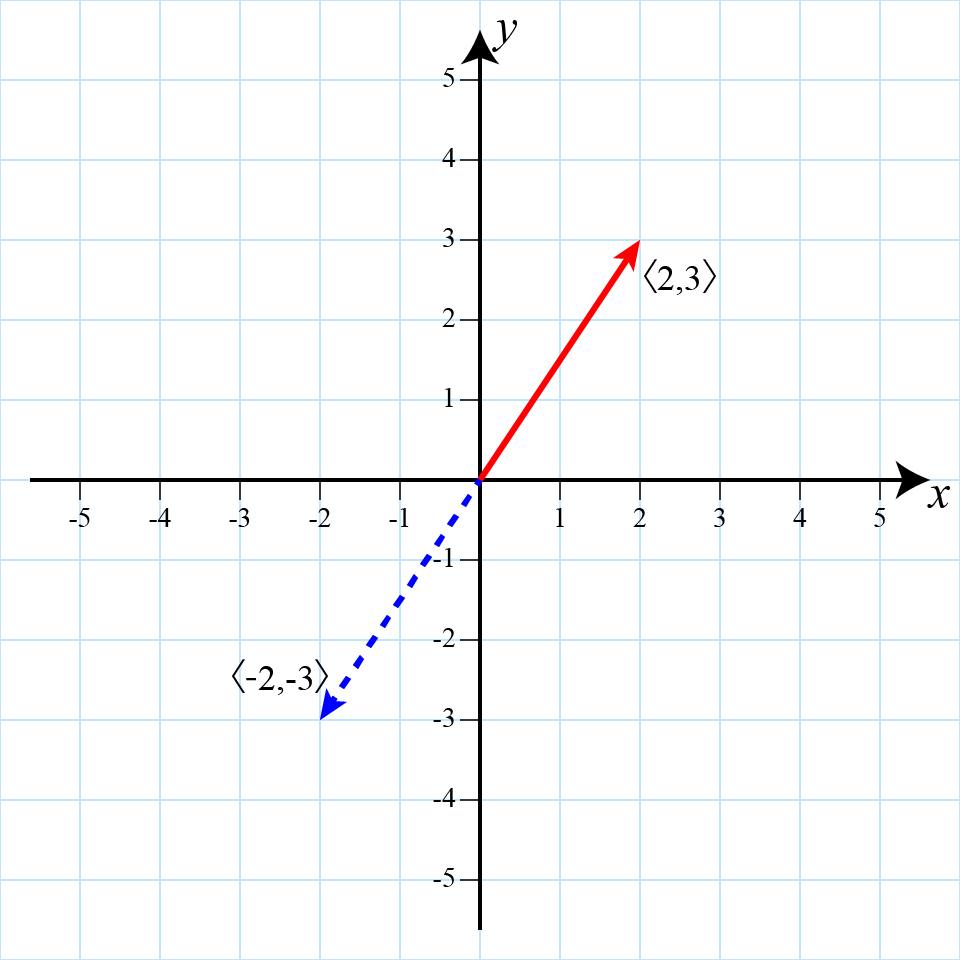
Reversing the direction of the red vector
Vectors themselves can also be combined to “put one after the other”. We call this operation “vector addition.” Visually it works by simply putting one arrow after the other:
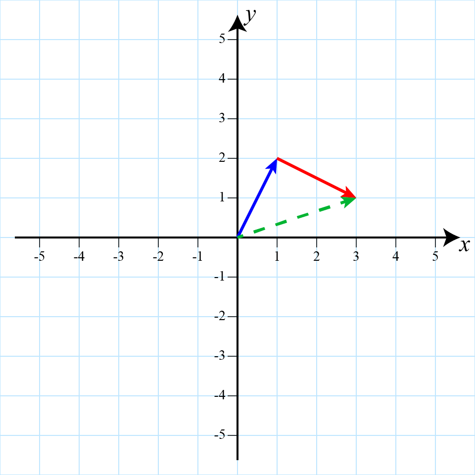
Adding the blue and red vectors, which produces the green vector.
Again, this operation makes sense because vectors are not tied to any position and can
move about freely. Mathematically, this operation is also very easy to implement if we
use the angle-brackets way of representing vectors: we just add the
One last operation useful operation is rotating a vector by an angle
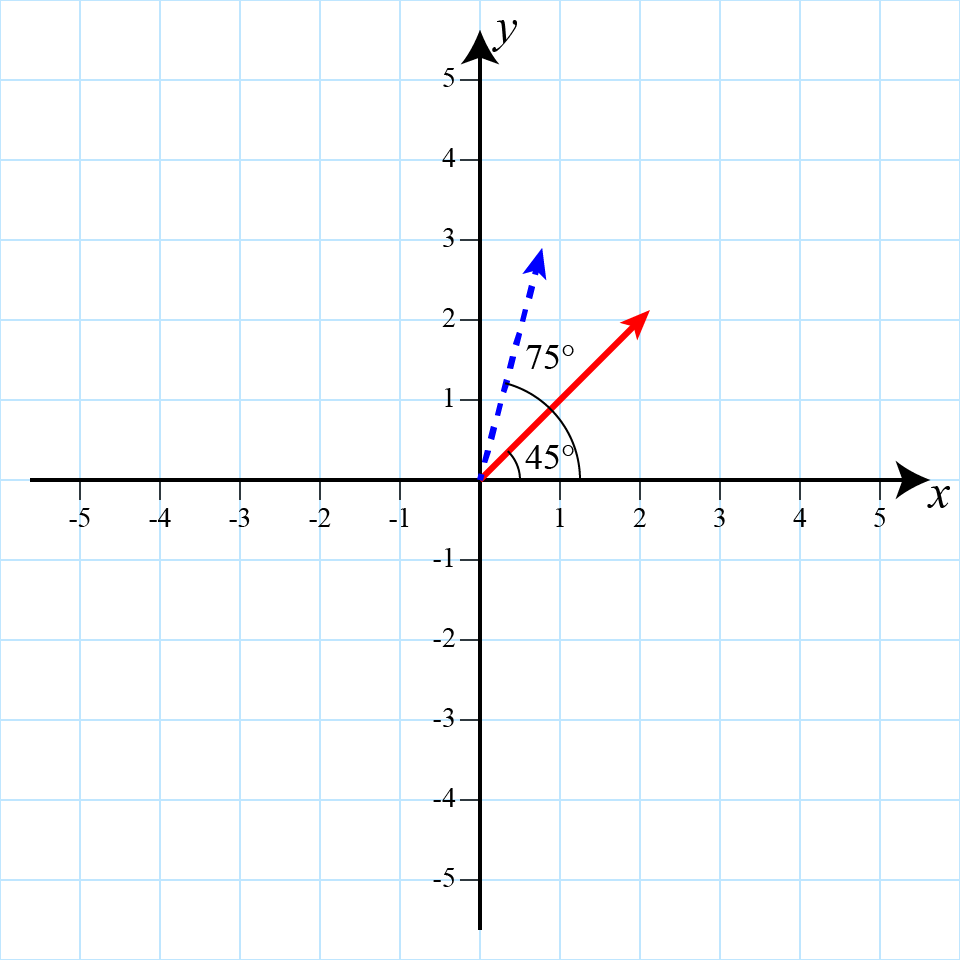
Rotation of the red vector by π/6 (30°)
Scalars
The last mathemetical concept to define is the scalar. A scalar is simply a single numeric value (in python terms, an int or float). However, scalars are important for physical systems because of how we can use them to manipulate vectors.
The primary use of a scalar is for scalar multiplication. Visually, multiplying a vector by a scalar simply extends that vector by multiplying its magnitude bythe scalar value:
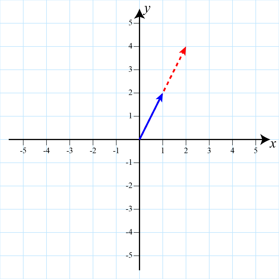
Multiplying the blue vector by 2 to create the dotted red vector.
Note that the direction of the vector does not change.
Scalar multiplication is simple in both vector representations:
Unit Vectors
While we often think of vectors in terms of direction and magnitude, the trigonometric formulas are complicated enough that we generally prefer to use the angle-bracket notation. Fortunately, scalar multiplication gives us another way to think of direction and magnitude.
A unit vector is a vector is a vector with length 1. If we take any vector
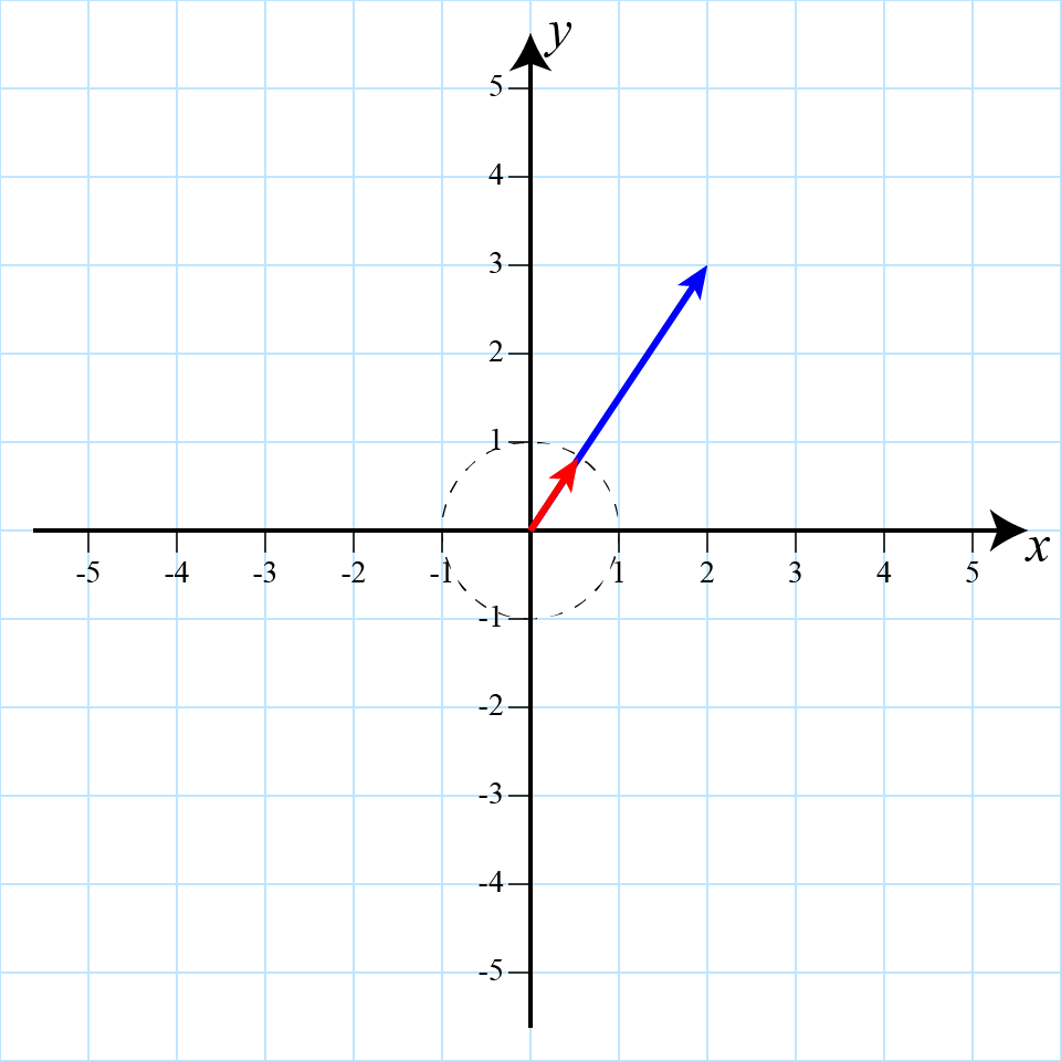
Computing the unit vector (red) for the blue vector.
As the direction of the unit vector is the same as the original vector, we typically use the unit vector to represent direction instead of the angle. So any vector is the scalar multiplication of its magnitude with its unit vector. A common operation in physics is to take a vector, convert it into a unit vector to get the direction, and then multiply that vector by a scalar to get a new vector.
Python Support
Scalars are naturally built into Python. The module introcs supports the classes
Point2 and
Vector2. The vector objects
are in angle-bracket notation with an
Vector2 and Point2 support operator overloading to implement many of the operations
above. We can use + to add to vectors. Adding a vector and point together applies the
vector, creating a new point at the resulting position. And we can multiply vectors by
ints or floats (scalar multiplication) either on the left or on the right.
Finally, Vector2 has methods for computing unit vectors. There is an
immutable version
that returns a new vector. There is also a
mutable version
that modifies the vector object itself. Note that neither of these methods work for the
zero vector, which is a vector with 0 magnitude.
