| P3.1 mode |
P3.2 square root |
P3.3 celestial motion |
P3.4 polynomials |
P3.5 vectorization |
P3.6 submission |
|---|
Completing all tasks in this assignment should teach you:
Modification History
| [2/17] Grayed out |
Topics: While loops, handling user input.
Setup: There are many different kinds of averages. Consider the sequence 9 3 1 5 1 2 7 5.
Task: Write a Matlab script readmode.m to read a sorted sequence of numbers entered one-by-one from the keyboard and store the leftmost mode in variable leftmostmode. The sequence ends when the user enters -1. Note that -1 is not part of the sequence. Leftmost means that if there are several modes, print the leftmost one (i.e. the one whose elements were typed earlier by the user). You may not use vectors of unbounded length. Use only scalars, structs, or vectors of length at most, say, 3.
The sequence can be either non-ascending or non-descending. Note that it is possible to write your program so that it doesn't know/care if the sequence is going up or down.
For example, if the user's input was 3, 7, 8, 8, 9, 9, 9, 13, 14, 17, 17, 17, -1, the program's answer should be 9. Think a minute about what should happen if -1 is the first number entered at the keyboard. Make sure that your program treats this situation gracefully and gives a reasonable response.
Turn in your script file. You may not define any functions or other scripts.
Note:The original question was too hard for now. It will probably be assigned later.
|
Setup: An arithmetic sequence is a sequence a, a+d, a+2d, a+3d, a+4d, ... where the gap d between successive numbers is constant. For example, 5, 5, 5, ... and 1, 3, 5, 7, 9, ... are arithmetic sequences, but 1, 3, 6, 10 is not. Task: Write a program to read a sequence of numbers entered one-by-one from the keyboard. The sequence ends when the user enters -1. Note that -1 is not part of the sequence. Print out the longest arithmetic subsequence that you can find in the input. If there are several arithmetic sequences of maximal lenth, print the leftmost one (i.e. the one whose elements were typed earlier by the user). For example, if the user's input was 1, 2, 0, 3, 6, 9, 12, 14, 7, 0, 2, 1, 0, -1, the program's answer should be [0 3 6 9 12]. Think a minute about what should happen if -1 is the first or the second number entered at the keyboard. Make sure that your program treats these situations gracefully and gives a reasonable response.
|
Bonus:
|
|
Topics: Formatted output, iterative numerical algorithms, convergence.
Setup: Given a function f(x), a value xp is called a fixed point for function f if and only if f(xp) = xp. Fixed points are very important in several areas of engineering and science. Finding them is often quite challenging.
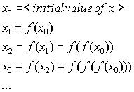
One way of finding fixed points is to start with an arbitrary value "close enough" to the solution and compute a series of values as follows:

In this problem we will be looking for the fixed points of the function

Task: Write a function [fp,k]=mysqrt(a,epsilon) to compute successive approximations of the fixed point. Start at x0=1. (Mathematically, any non-zero starting value is fine, including negative numbers. Numerically (i.e. on a computer), just about any non-zero starting value will work.) Continue the iterations until the absolute value (type help abs for details) of the difference between two successive approximations, say xk and xk+1, is less than the given tolerance epsilon. The value xk+1 determined will be considered the correct value fp of the fixed point.
Write a Matlab script testmysqrt.m to test your function for each of the following values of the parameter a: 3, 4, 5, and 9. Use epsilon=10-6. For each run print the following information formatted exactly as below:
Value of parameter a is: <value of a shown with 6 decimals>.
Value of fixed point: <value of fixed point with 8 decimals>.
Number of iterations: <value of index k+1 printed as an integer>.
Leave exactly one empty row between the lines which provide results for a given value of paramerer a.
Turn in your function and script. You may not define other scripts or functions.
HINT: You will probably find it useful to learn about functions sprintf, disp, num2str, str2num when working on this assignment.
Topics: Plotting 2D curves, approximate solution to differential equations.
Setup: In this problem we will simulate and study the behavior of celestial objects under the influence of gravitation. Let us consider a massive star (S) in the origin of a system of coordinates XY. A small comet C can be found at position x0 = R0, y0 = 0, and has currently a speed of v0 parallel to axis y and oriented toward its positive direction. The diagram below illustrates the just described initial conditions:
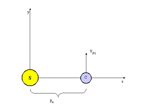
The gravitational force that acts on the comet is oriented along the line which unites the center of the comet with the center of the star, and it is oriented toward the star. This force will accelerate the comet toward the star.
If the comet had no radial speed, it would fall straight into the star. If it has a non-zero radial speed, as in this problem, the comet will describe a trajectory whose characteristics depend on the initial conditions. In this latter case the comet will in general change its distance from S, but it will also move (at least partially) around it.
If we know the position (xt, yt) of the comet at moment t, we can describe the comet's movement by using differential equations. It is best if we separate the movements along the two axes, and we study them separately. We get the following two equations:
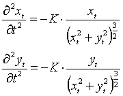
Remember that the derivative of a function is just the ratio of the function's change and the corresponding change in its argument, when the argument's change is gradually decreased to 0. When using finite diferences we don't compute the limit of this ratio, but we stop at a "small enough" value for the change in the function argument and take the corresponding ratio as a good approximation of the true result. Finite difference methods work well if the solution sought is a "well-behaved" function, and if the difference in the the function arguments is kept "small enough." These terms have much more precise mathematical definitions, but we can ignore details in our discussion.
In the two differential equations at hand it is the time variable that we have to discretize. We will call the time interval taken as change in the function argument (or independent variable) Dt. We will compute the acceleration the comet is subject to only at discrete points in time, each separated by Dt. We will assume that the gravitational force and the acceleration determined by it does not change in this interval. It is easy to admit intuitively that the smaller Dt is, the less the gravitational force can change in that interval, and the better our approximation will be. In practice we can't take Dt to be very small, because at that level the inherent imprecision of numerical computations creates other problems; do you remember the approximations of e=2.7183...?
After discretization we obtain the following equations for the comet's movement:
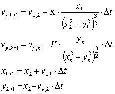
Task: Write a function [x,y]=celestial(K,dt,R0,v0,N,skip) that simulates the movement of the comet around the star by tracking the changes in its x and y coordinates for N steps. Out of the N+1 pairs of coordinates, return only every skip-th pair, beginning with the starting point.
[2/15] Note:
(Some versions of?) the Student Edition of Matlab impose a limit of of 16384 elements in an array. This means for large values of N you cannot store all N+1 pairs of coordinates and then select out only the ones you want: you must selectively store elements as you go. Even without such a limit, it would have been a good idea not to store data that will be thrown out anyway: it is wasteful of memory. HINT: if you use a for loop from 0 to N, observe that the remainders when you divide the loop variable by skip are periodic, e.g. equal to 0 only once every skip loop iterations.
Write a script testcelestial.m to perform simulations for the following cases:
|
In your script, use statement plot(X,Y) to display the comet's
trajectory |
| Turn in your function and script. |
| Make sure each plot has a descriptive title. |
Topics: Functions, array manipulations, error-checking.
Setup: Many computational problems are ultimately solved using polynomials, even if the theoretical (i.e. purely mathematical) solutions don't even refer to them. One reason for this is that very often it is impossible, or impractical, to directly handle the very complex functions that theoretical methods involve. Because almost all functions important in practice can be approximated with any desired precision by using polynomials, they are very often used to simplify the original problem and make the finding of an approximate solution feasable.
Although Matlab does provide support for polynomials, most programming languages do not. This provides us with an opportunity. In case you need to manipulate polynomials in a programming language that does not support them, your role in this part is to implement a set of functions that manipulate polynomials. The skills you learn will apply to just about any programming language you are likely to encounter. Since Matlab already provides support, this is a means for you to compare your answers with Matlab's.
We will represent polynomials by using arrays. Polynomial an*xn+an-1*xn-1+...+a2*x2+a1*x+a0 will be represented by the array [a0, a1, a2, ..., an-1, an].
Note that the array stores the coefficients in right-to-left order. Matlab, however, stores coefficients in left-to-right order; therefore, to convert between our representation and Matlab's, you should use the fliplr function. To make the polynomial representation unique, we will impose the condition that the representation be in canonical form: the leading coefficient an (last number in the vector) must be non-zero for all polynomials except the constant polynomial 0.
We will consider the following operations for/on polynomials: creation, addition, subtraction, multiplication, division, and evaluation. Remember that polynomial divisions typically generate a remainder. (See Examples below.)
Since part of programming is debugging and testing, we will ask you to write a Matlab script file that performs some tests to check that your implementation works.
Task: Implement Matlab functions for all the operations mentioned above and a Matlab script file that tests your functions. Except for makepoly, your functions may assume their arguments are in canonical form. The respective functions and script should have the arguments and behavior specified below:
| Function Name | Required Functionality |
|---|---|
| makepoly (p) | Compute canonical form for polynomial p: strip off "leading" 0s (trailing 0s in the vector). |
| addpoly (p1, p2) | Compute and return p2+p1. |
| subpoly (p1, p2) | Compute and return p2-p1. |
| mulpoly (p1, p2) | Compute and return the multiplication of polynomial p1 and p2.
Note: do not type the strings conv or deconv anywhere in your function file. |
| divpoly (p1, p2) | Compute and return the quotient and remainder of dividing p1
by p2. When called with one return argument (e.g. q=
divpoly(p1, p2)) the function should return the quotient
only. When called with two arguments (e.g. [q r] = divpoly(p1,
p2)), the function should return the quotient and the
remainder in the first and second argument, respectively.
Note: do not type the strings conv or deconv anywhere in your function file. |
| evalpoly (p, x0) | Compute and return value of polynomial p at point x0. |
| Script Name | Required Functionality |
| testpoly | Run various tests and checks on your functions. Give enough examples to be convincing, but not too many. Spend some time thinking of how to choose relevant examples only. Include degenerate cases, but otherwise avoid trivial examples. Include comparisons with Matlab's polynomial functions: polyval, conv, deconv. |
Turn in the functions and script listed above. You may not define other functions or scripts.
HINT: Ask on help for nargout. TKY didn't, but you might find it useful for this assignment.
Examples:
Topics: Vectorizing code
Setup: The emphasis on Project P2 and Prelim T1 was on problem solving and correctness. Let us now consider conciseness. In particular, let us consider how to vectorize code for problems we have already seen to reduce the use of loops.
Task: Write and turn in the 5 separate Matlab scripts specified below without using any loops or user-defined functions.
The online submission system is up. Make sure to include the information requested in the Submission Rules. Your script and function files may not start with a space or blank line: Your script files must start with a comment and your function files must start with the function keyword (place the required identification comment block (you and your partner's name, cuid, section, etc.) below the comment specifying the behavior of the function).
You may submit files as you complete them. You don't have to submit everything all at once.
Please post/e-mail about any problems you have so that we can quickly fix things.
Note: Many people on Project P2 made up their own variable names; doing that on P3 will cost you points. Make sure to use verbatim (spelling, upper-/lowercase, etc.) the function and variable names we specify. (Script names on P3 don't have to match.)
Early Bonus: We will award bonus points for submitting the entire project early: No early bonus points for partial submissions.