Lecture 2: k-nearest neighbors

Processing math: 100%

Lecture 2: k-nearest neighbors

back

The k-NN algorithm

Assumption: Similar Inputs have similar outputs
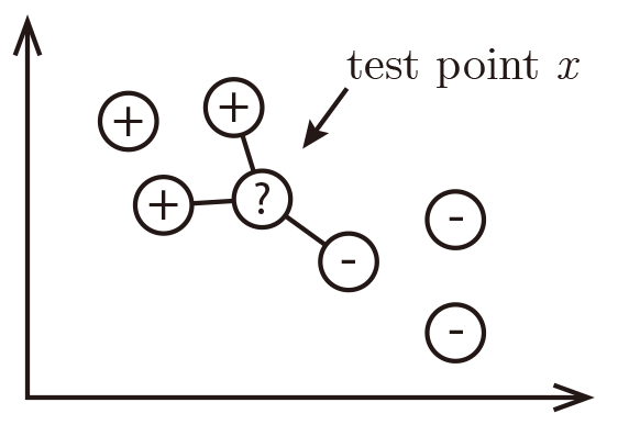
Classification rule: For a test input

$x$ , assign the most common label amongst its k most similar training inputs

Neighbors' labels are $2\times$ ⊕ and $1\times$ ⊖ and the result is ⊕.

Formal (and borderline incomprehensible) definition of k-NN:

Test point:

$\mathbf{x}$

Define the set of the

$k$ nearest neighbors of

$\mathbf{x}$ as

$S_\mathbf{x}$ . Formally

$S_\mathbf{x}$ is defined as

$S_\mathbf{x}\subseteq {D}$ s.t.

$|S_\mathbf{x}|=k$ and

$\forall(\mathbf{x}',y')\in D\backslash S_\mathbf{x}$ ,

$\text{dist}(\mathbf{x},\mathbf{x}')\ge\max_{(\mathbf{x}'',y'')\in S_\mathbf{x}} \text{dist}(\mathbf{x},\mathbf{x}''),$ (i.e. every point in

$D$ but not in

$S_\mathbf{x}$ is at least as far away from

$\mathbf{x}$ as the furthest point in

$S_\mathbf{x}$ ). We can then define the classifier

$h()$ as a function returning the most common label in

$S_\mathbf{x}$ :

$h(\mathbf{x})=\text{mode}(\{y'':(\mathbf{x}'',y'')\in S_\mathbf{x}\}),$ where

$\text{mode}(\cdot)$ means to select the label of the highest occurrence.

(Hint: In case of a draw, a good solution is to return the result of

$k$ -NN with smaller

$k$ )

What distance function should we use?

The k-nearest neighbor classifier fundamentally relies on a distance metric. The better that metric reflects label similarity, the better the classified will be. The most common choice is the Minkowski distance

$\text{dist}(\mathbf{x},\mathbf{z})=\left(\sum_{r=1}^d |x_r-z_r|^p\right)^{1/p}.$
Quiz#1: This distance definition is pretty general and contains many well-known distances as special cases:

$p = 1$ : Manhattan Distance (

$l_1$ -norm)

$p = 2$ : Euclidean Distance (

$l_2$ -norm)

$p \to \infty$ : Maximum Norm

$p \to 0$ : (not well defined)

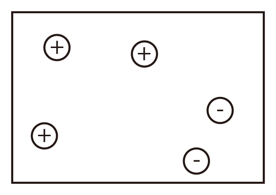
Quiz#2: How does

$k$ affect the classifier? What happens if

$k=n$ ? What if

$k =1$ ?

$k = n$

$k = 1$

Brief digression (Bayes optimal classifier)

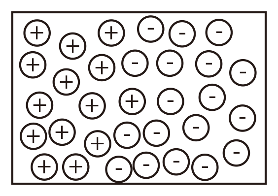
What is the Bayes optimal classifier? Assume you knew

$\mathrm{P}(y|\mathbf{x})$ . What would you predict?
Examples:

$y\in\{0,1\}$

$\mathrm{P}(+1| x)=0.8\\ \mathrm{P}(-1| x)=0.2\\ \text{Best prediction: }y^* = h_\mathrm{opt} = argmax_y P(y|\mathbf{x})$ (You predict the most likely class.) What is the error of the BayesOpt classifier?

$\epsilon_{BayesOpt}=1-\mathrm{P}(h_\mathrm{opt}(\mathbf{x})|y) = 1- \mathrm{P}(y^*|\mathbf{x})$ (In our example, that is

$\epsilon_{BayesOpt}=0.2$ .) You can never do better than the Bayes Optimal Classifier.

1-NN Convergence Proof

Cover and Hart 1967^[1]: As $n \to \infty$ , the $1$ -NN error is no more than twice the error of the Bayes Optimal classifier. (Similar guarantees hold for

$k>1$ .)

$n$ small

$n$ large

$n\to\infty$

Let

$\mathbf{x}_\mathrm{NN}$ be the nearest neighbor of our test point

$\mathbf{x}_\mathrm{t}$ . As

$n \to \infty$ ,

$\text{dist}(\mathbf{x}_\mathrm{NN},\mathbf{x}) \to 0$ , i.e.

$\mathbf{x}_\mathrm{NN} \to \mathbf{x}_{t}$ . (This means the nearest neighbor is identical to

$\mathbf{x}_\mathrm{t}$ .) You return the label of

$\mathbf{x}_\mathrm{NN}$ . What is the probability that this is not the label of

$\mathbf{x}$ ? (This is the probability of drawing two different label of

$\mathbf{x}$ )

$\begin{multline*} \epsilon_{NN}=\mathrm{P}(y^* | \mathbf{x}_{t})(1-\mathrm{P}(y^* | \mathbf{x}_{NN})) + \mathrm{P}(y^* | \mathbf{x}_{NN})(1-\mathrm{P}(y^* | \mathbf{x}_{t}))\\ \le (1-\mathrm{P}(y^* | \mathbf{x}_{NN})+(1-\mathrm{P}(y^* | \mathbf{x}_{t}) = 2(1-\mathrm{P}(y^* | \mathbf{x}_{t}) = 2\epsilon_\mathrm{BayesOpt}, \end{multline*}$ where the inequality follows from

$\mathrm{P}(y^* | \mathbf{x}_{+})\le 1$ and

$\mathrm{P}(y^* | \mathbf{x}_{NN})\le 1$ .

In the limit case, the test point and its nearest neighbor are identical. There are exactly two cases when a misclassification can occur: when the test point and its nearest neighbor have different labels. The probability of this happening is the probability of the two red events: $(1\!-\!p(s|\mathbf{x}))p(s|\mathbf{x})+p(s|\mathbf{x})(1\!-\!p(s|\mathbf{x}))=2p(s|\mathbf{x})(1-p(s|\mathbf{x}))$

Good news: As

$n \to\infty$ , the

$1$ -NN classifier is only a factor 2 worse than the best possible classifier.
Bad news: We are cursed!!

Curse of Dimensionality

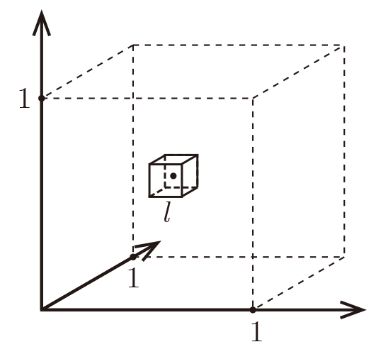
Imagine

$X=[0,1]^d$ , and

$k = 10$ and all training data is sampled uniformly with

$X$ , i.e.

$\forall i, x_i\in[0,1]^d$

Let

$\ell$ be the edge length of the smallest hyper-cube that contains all

$k$ -nearest neighbor of a test point. Then

$\ell^d\approx\frac{k}{n}$ and

$\ell\approx\left(\frac{k}{n}\right)^{1/d}$ . If

$n= 1000$ , how big is

$\ell$ ?

$d$		$\ell$
2		0.1
10		0.63
100		0.955
1000		0.9954

Almost the entire space is needed to find the

$10$ -NN.

Figure demonstrating ``the curse of dimensionality''. The histogram plots show the distributions of all pairwise distances between randomly distributed points within $d$ -dimensional unit squares. As the number of dimensions $d$ grows, all distances concentrate within a very small range.

Imagine we want

$\ell$ to be small (i.e the nearest neighbor are truly near by), then how many data point do we need? Fix

$\ell=\frac{1}{10}=0.1$

$\Rightarrow$

$n=\frac{k}{\ell^d}=k\cdot 10^d$ , which grows exponentially!
Rescue to the curse: Data may lie in low dimensional subspace or on sub-manifolds. Example: natural images (digits, faces).

k-NN summary

$k$ -NN is a simple and effective classifier if distances reliably reflect a semantically meaningful notion of the dissimilarity. (It becomes truly competitive through metric learning)

$n \to \infty$ ,

$k$ -NN becomes provably very accurate, but also very slow.

$d \to \infty$ , the curse of dimensionality becomes a concern.

Reference

[1]Cover, Thomas, and, Hart, Peter. Nearest neighbor pattern classification[J]. Information Theory, IEEE Transactions on, 1967, 13(1): 21-27